W#06: Principal Component Analysis, Math: Exponentiations and Logarithms, Epidemic Modeling, Calculus
Two Variables
Example for the new axes.
Code
pca1 <- peng |> select(flipper_length_mm, bill_length_mm) |>
 prcomp(~., data = _, scale = FALSE)
pca_vec <- t(pca1$rotation) |> as_tibble() # Vectors with x = flipper_length, y = bill_length
ggplot(peng) +
 geom_point(aes(x = flipper_length_mm, y = bill_length_mm, color = species)) +
 geom_segment(
  data = pca_vec,
  aes(x = mean(peng$flipper_length_mm),
      y = mean(peng$bill_length_mm),
      xend = c(pca1$sdev)*flipper_length_mm + mean(peng$flipper_length_mm),
      yend = c(pca1$sdev)*bill_length_mm + mean(peng$bill_length_mm)),
  arrow = arrow(length = unit(0.3, "cm"))) +
 coord_fixed()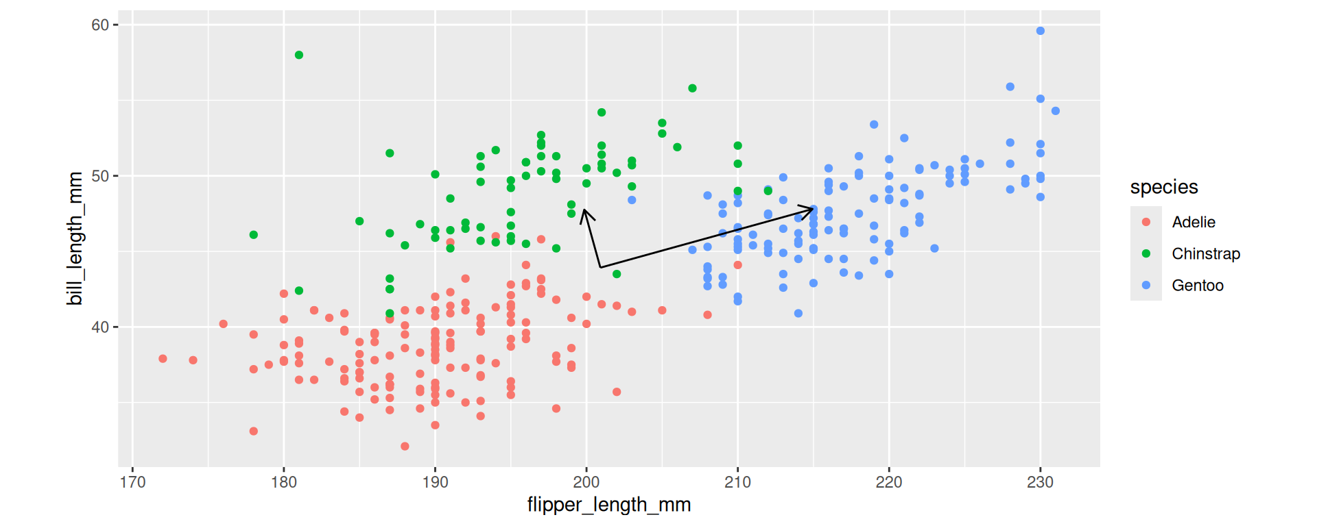
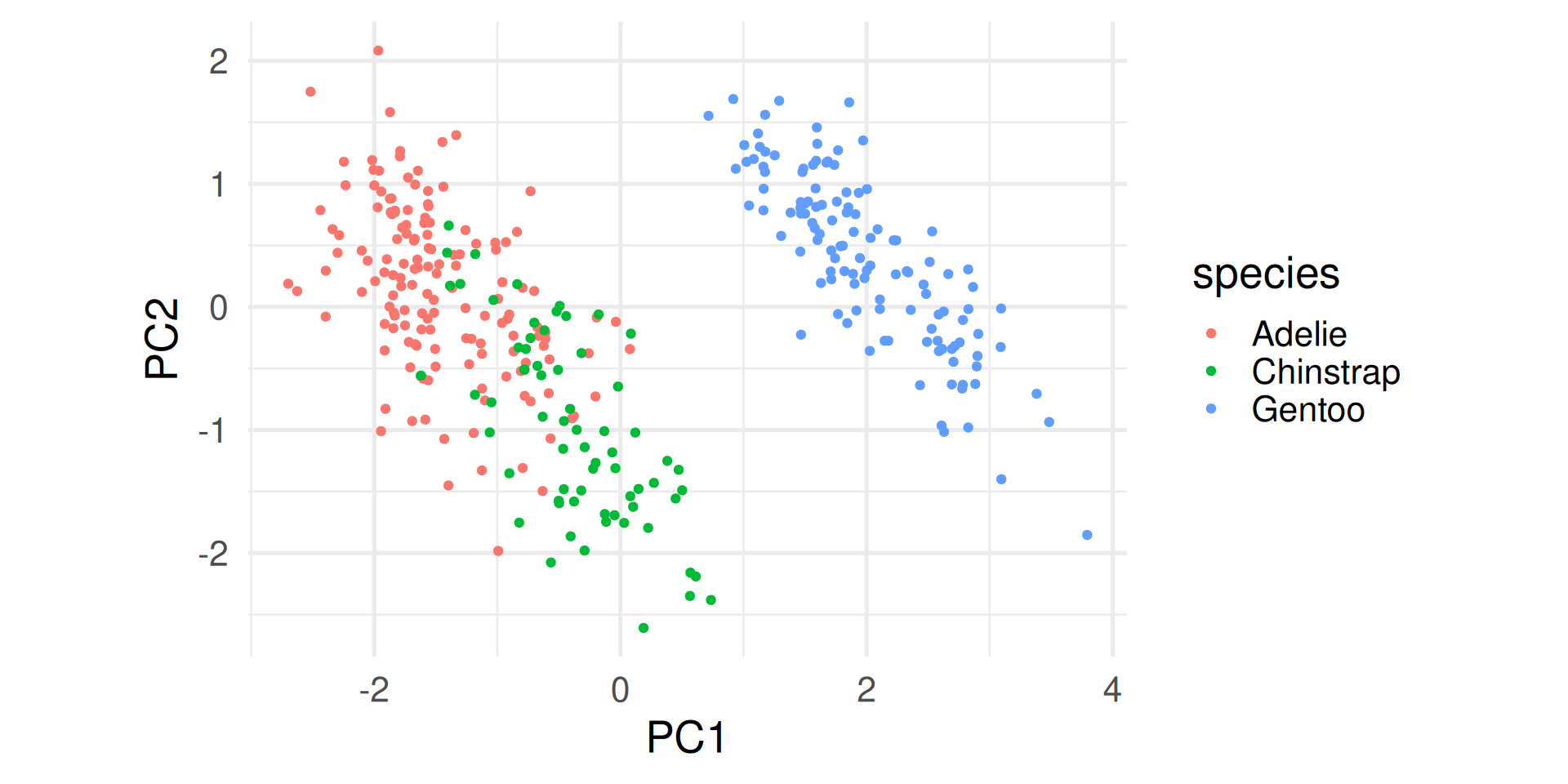
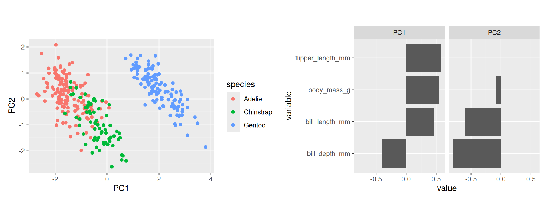
Explore data in PC coordinates
- Start plotting PC1 against PC2. By default these are the most important ones. Drill deeper later.
- Append the original data. Here used to color by species.
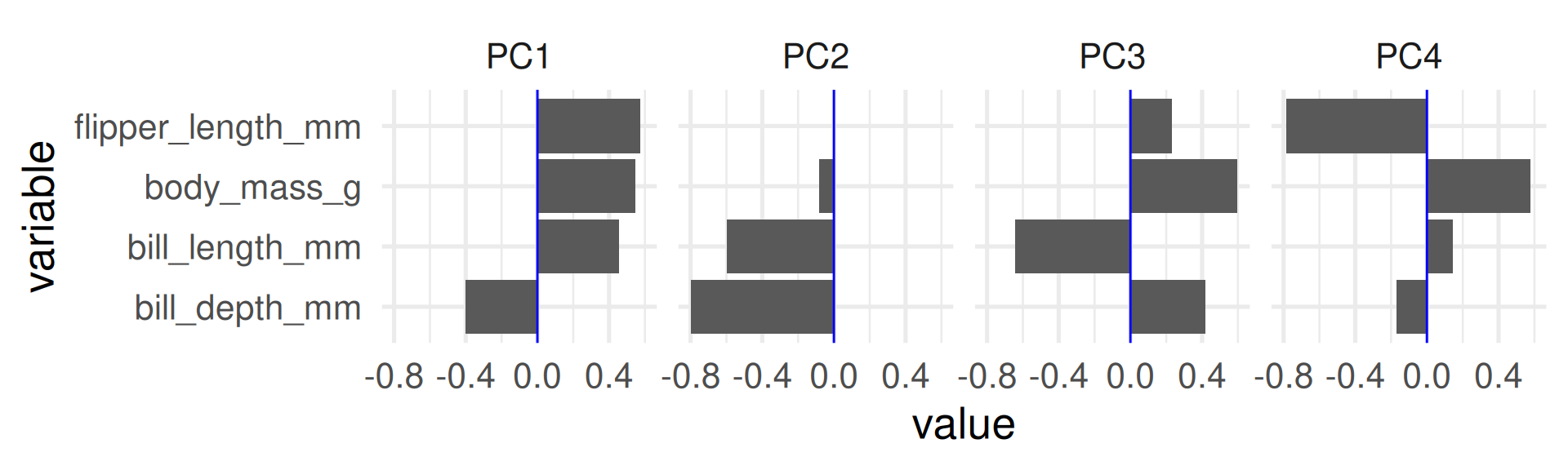
Variable loadings
- The columns of the rotation matrix shows how the original variables load on the principle components.
- We can interpret these loadings and give descriptive names to principal components.
- For plotting we bring the rotation matrix to long format with
PCandvaluecolumn.
Variance explained
- Principle components are by default sorted by importance.
- The squares of the standard deviation for each component gives its variances and variances have to sum up to the sum of the variances of the original variables.
- When original variables were standardized their original variances are all each one. Consequently, the variances of the principal components sum up to the number of original variables.
- A typical plot to visualize the importance of the components is to plot the percentage of the variance explained by each component.
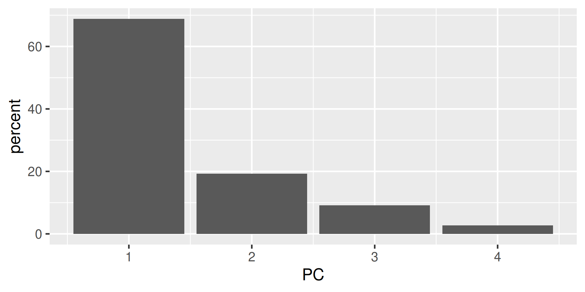
Interpretations (1)
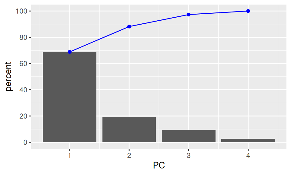
- The first component explains almost 70% of the variance.
- The first two explain about 88% of the total variance.
Interpretations (2)
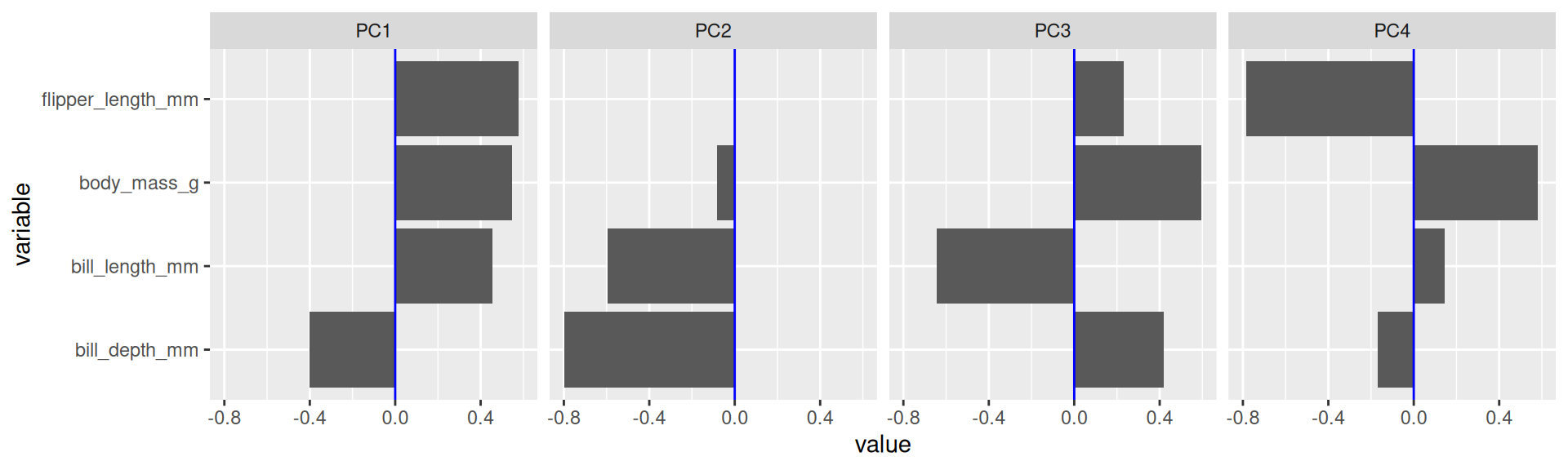
- To score high on PC1 a penguin needs to be generally large but with low bill depth.
- Penguins scoring high on PC2 are penguins with generally small bills.
Interpretations (3)


Relations of PCA
- A technique similar in spirit is factor analysis (e.g.
factanal). It is more theory based as it requires to specify to the theoriezed number of factors up front. - PCA is an example of the importance of linear algebra (“matrixology”) in data science techniques.
- PCA is based on the eigenvalue decomposition of the covariance matrix (or correlation matrix in the standardized case) of the data.

More rules for exponentiation
\(x^a\cdot x^b\)
\(x^a\cdot x^b = x^{a+b}\) Multiplication of powers (with same base \(x\)) becomes addition of exponents.
\((x+y)^a\)
No “simple” form! For \(a\) integer use binomial expansion. \((x+y)^2 = x^2 + 2xy + y^2\)
\((x+y)^3 = x^3 + 3x^2y + 3xy^2 + y^3\)
\((x+y)^n = \sum_{k=0}^n {n \choose k} x^{n-k}y^k\)
Pascal’s triangle

We meet it again in Probability:
A row represents a binomial distribution
Which tends to mimics the normal distribution more and more
and is related to the central limit theorem
SIR model
- Assume a population of \(N\) individuals.
- Individuals can have different states, e.g.: Susceptible, Infectious, Recovered, …
- The population divides into compartments of these states which change over time, e.g.: \(S(t), I(t), R(t)\) number of susceptible, infectious, recovered individuals
Now we define dynamics like
where the numbers on the arrows represent transition probabilities.
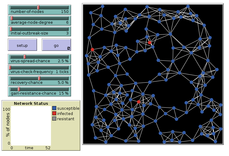
Agent-based Simulation
Agent-based model: Individual agents are simulated and interact with each other.
Explore and analyze with computer simulations.
A tool: NetLogo https://ccl.northwestern.edu/netlogo/

We look at the model “Virus on a Network” from the model library.
Direct Link to Virus on a Network in NetLogoWeb
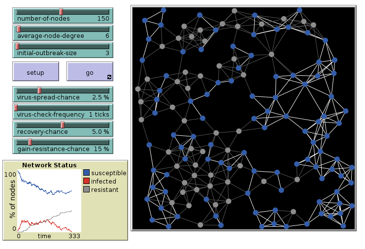
Virus on a Network: 6 links, initial
Agents connected in a network with on average 6 links per agent. 3 are infected initially.
Virus on a Network: 6 links, final
The outbreak dies out after some time.
Virus on a Network: 15 links, initial
Repeat the simulation with 15 links per agent. 3 are infected initially. 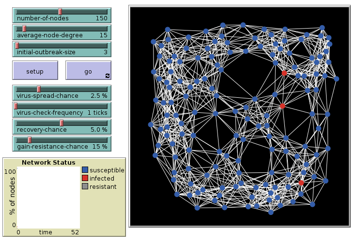
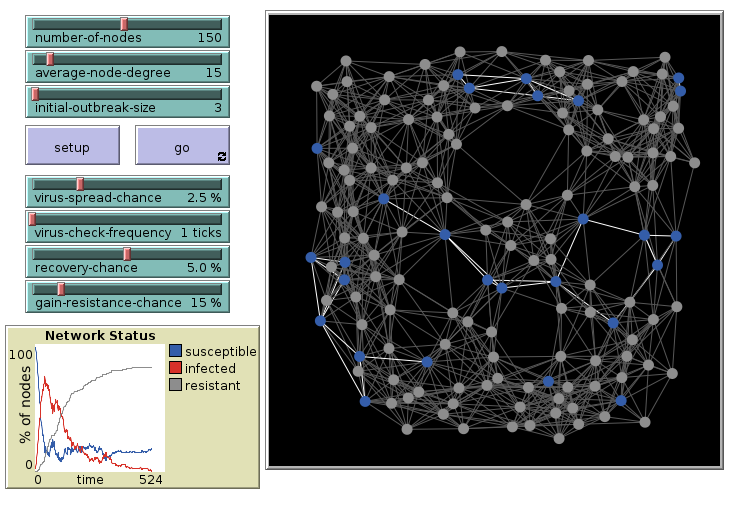
Virus on a Network: 15 links, final
The outbreak had infected most agents.
SI-model: Simulation in R
Iteration over 75 time steps.
tmax <- 75
sim_run <- list(init) # list with one element
# This list will collect the states of
# all individuals over tmax time steps
for (i in 2:tmax) {
 # Every agents has a contact with a random other
 contacts <- sample(sim_run[[i-1]], size = N)
 sim_run[[i]] <- if_else( # vectorised ifelse
  # conditions vector: contact is infected
  # and a random infection happens
  contacts == "I" & randomly_infect(N, beta),
  true = "I",
  false = sim_run[[i-1]]
  ) # otherwise state stays the same
}
sim_output <- tibble( # create tibble for ggplot
 # Compute a vector with length tmax
 # with the count of "I" in sim_run list
 t = 0:(tmax-1), # times steps
 # count of infected and output a vector
 infected = sim_run |> map_dbl(\(x) sum(x == "I")))
sim_output |>
 ggplot(aes(t,infected)) + geom_line() +
 theme_minimal(base_size = 20)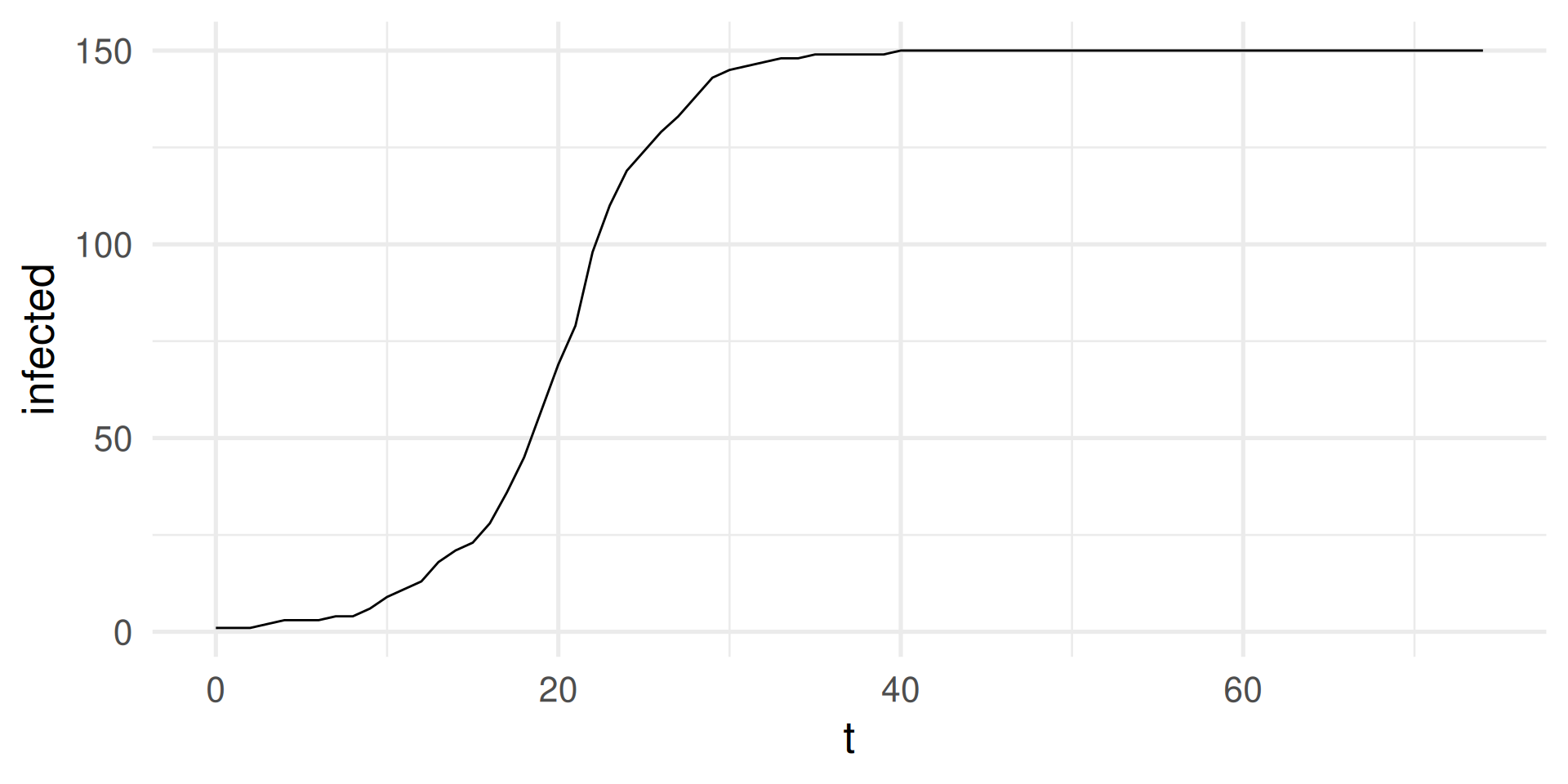
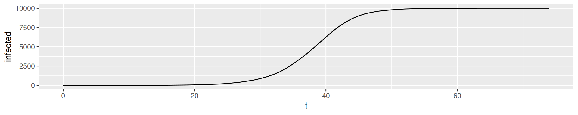
SI-model: Simulation in R
Run with \(N = 10000\)
N <- 10000
init <- rep("S",N) # All susceptible
init[1] <- "I" # Infect one individual
tmax <- 75
sim_run <- list(init) # list with one element
# This list will collect the states of
# all individuals over tmax time steps
for (i in 2:tmax) {
 # Every agents has a contact with a random other
 contacts <- sample(sim_run[[i-1]], size = N)
 sim_run[[i]] <- if_else( # vectorised ifelse
  # conditions vector: contact is infected
  # and a random infection happens
  contacts == "I" & randomly_infect(N, beta),
  true = "I",
  false = sim_run[[i-1]]
  ) # otherwise state stays the same
}
sim_output <- tibble( # create tibble for ggplot
 # Compute a vector with length tmax
 # with the count of "I" in sim_run list
 t = 0:(tmax-1), # times steps
 # count of infected, notice map_dbl
 infected = map_dbl(sim_run, \(x) sum(x == "I")))
sim_output |>
 ggplot(aes(t,infected)) + geom_line() +
 theme_minimal(base_size = 20)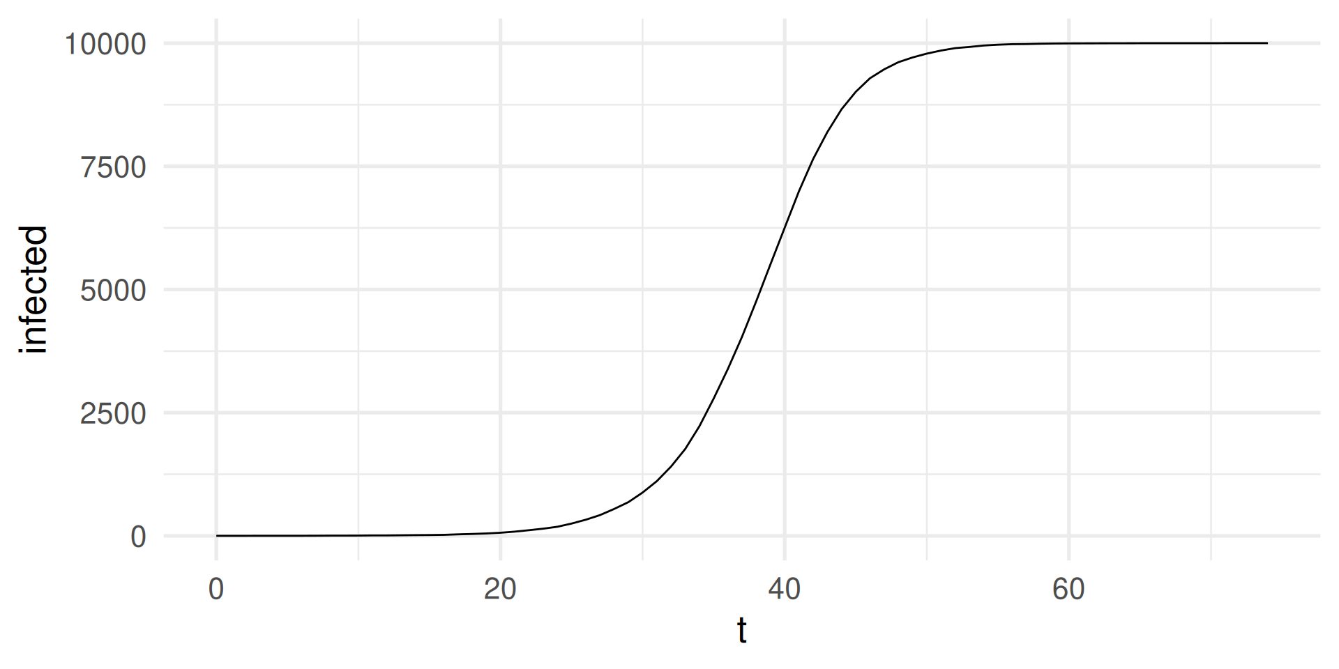
Derivatives
- The derivative of a function is also a function with the same domain.
- Measures the sensitivity to change of the function output when the input changes (a bit)
- Example from physics: The derivative of the position of a moving object is its speed. The derivative of its speed is its acceleration.
- Graphically: The derivative is the slope of a tangent line of the graph of a function.
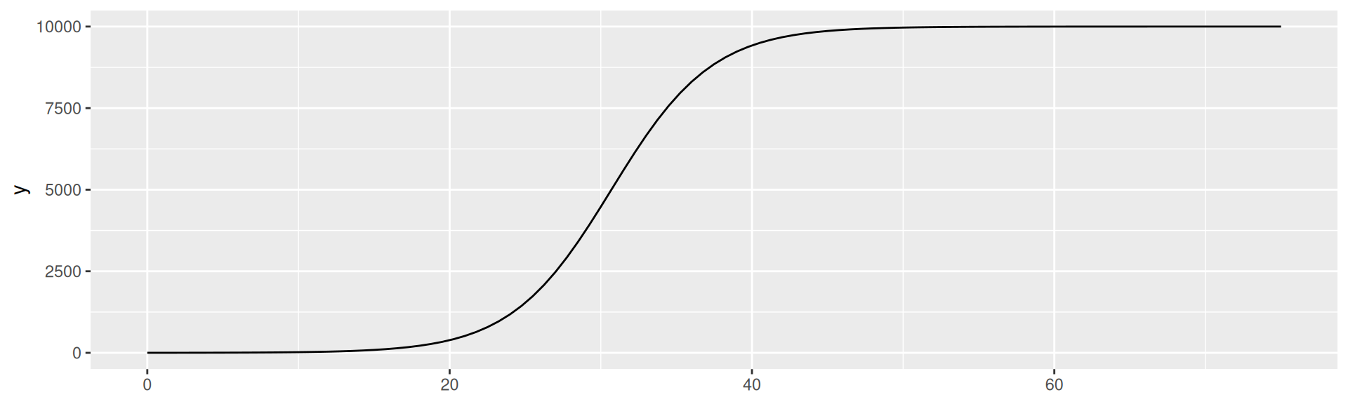
SI-model: Logistic Equation
\(I(t) = \frac{N}{1 + (\frac{N}{I(0)} - 1)e^{-\beta t}}\)
Plot the equation for \(N = 10000\), \(I_0 = 1\), and \(\beta = 0.3\)
SI-model: Numerical integration
Another way of solution is numerical integration, e.g. using Euler’s method.
We compute the solution step-by-step using increments of, e.g. \(dt = 1\).
N <- 10000
I0 <- 1
dI <- function(I,N,b) b*I*(N - I)/N
beta <- 0.3
dt <- 1 # time increment,
# supposed to be infinitesimally small
tmax <- 75
t <- seq(0,tmax,dt)
# this is the vector of timesteps
It <- I0 # this will become the vector
# of the number infected I(t) over time
for (i in 2:length(t)) {
 # We iterate over the vector of time steps
 # and incrementally compute It
 It[i] = It[i-1] + dt * dI(It[i-1], N, beta)
 # This is called Euler's method
}
tibble(t, It) |> ggplot(aes(t,It)) +
 geom_line(color = "red") +
 geom_function(
  fun = function(t) N / (1 + (N/I0 - 1)*exp(-beta*t)), color = "blue") +
 # In blue: Analytical solution for comparison
 theme_minimal(base_size = 20)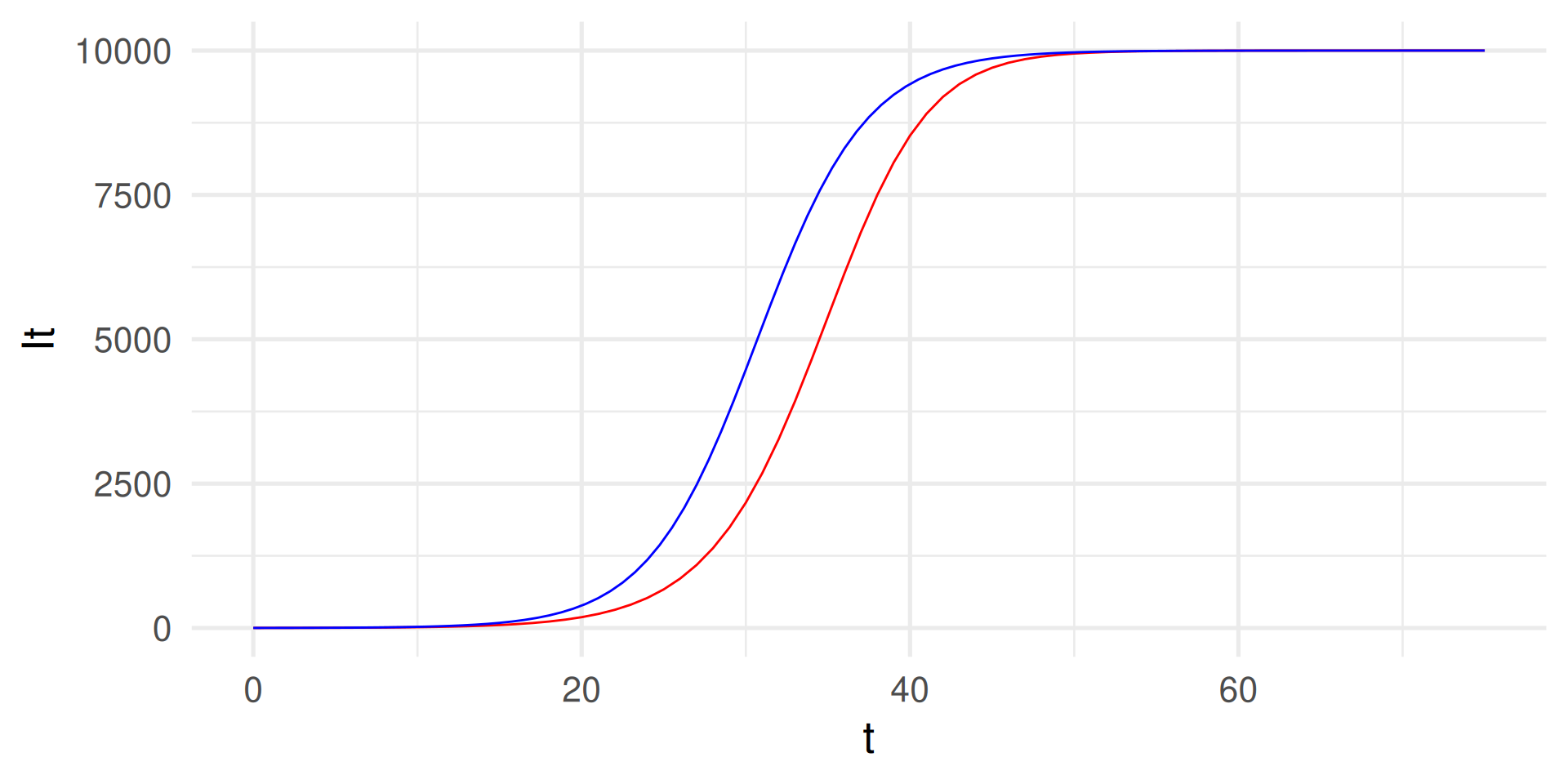
Why do the graphs deviate? The step size \(dt\) must be “infinitely” small
Numerical integration with smaller \(dt\)
We compute the solution step-by-step using small increments of, e.g. \(dt = 0.05\).
N <- 10000
I0 <- 1
dI <- function(I,N,b) b*I*(N - I)/N
beta <- 0.3
dt <- 0.05 # time increment,
# supposed to be infinitesimally small
tmax <- 75
t <- seq(0,tmax,dt)
# this is the vector of timesteps
It <- I0 # this will become the vector
# of the number infected I(t) over time
for (i in 2:length(t)) {
 # We iterate over the vector of time steps
 # and incrementally compute It
 It[i] = It[i-1] + dt * dI(It[i-1], N, beta)
 # This is called Euler's method
}
tibble(t, It) |> ggplot(aes(t,It)) +
 geom_line(color = "red") +
 geom_function(
  fun = function(t) N / (1 + (N/I0 - 1)*exp(-beta*t)), color = "blue") +
 # In blue: Analytical solution for comparison
 theme_minimal(base_size = 20)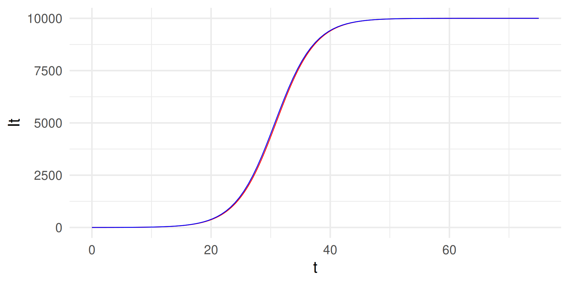
The diff of our simulation output
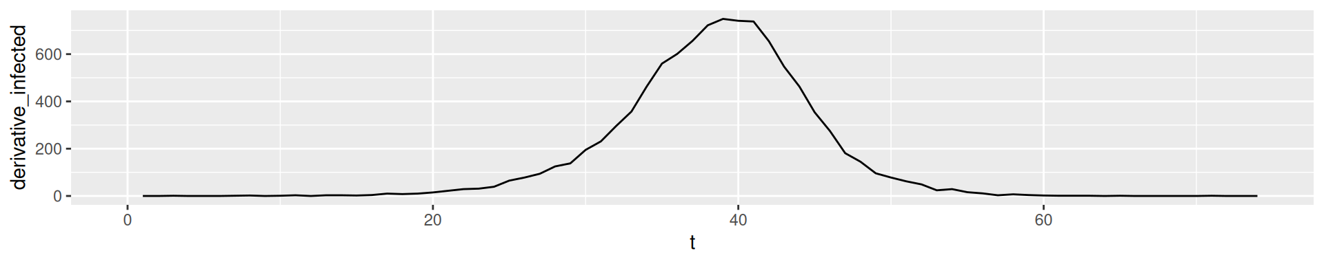
2nd derivative: Change of change
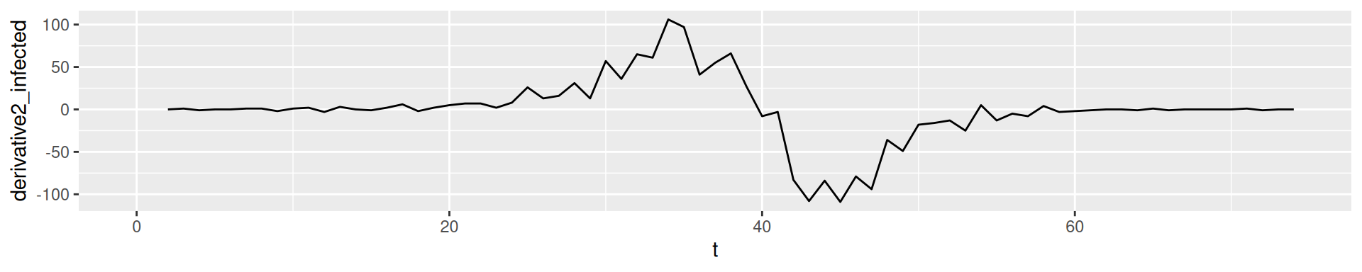
In empirical data: Derivatives of higher order tend to show fluctuation
Interpretation in SI-model
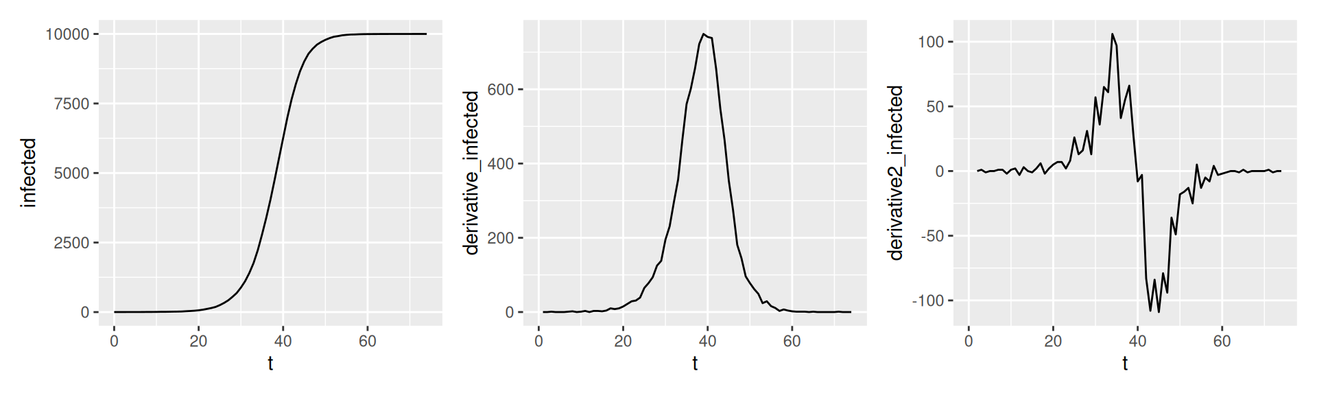
- \(I(t)\) total number of infected
- \(I'(t)\) number of new cases per day (time step)
- \(I''(t)\) how the number of new cases has changes compared to yesterday
- 2nd derivatives are a good early indicator for the end of a wave.
The fundamental theorem of calculus
The integral of the derivative is the function itself.
This is not a proof but shows the idea:
[1] 1 3 7 12 17 20 20[1] 1 2 4 5 5 3 0[1] 1 2 1 0 -2 -3[1] 1 2 4 5 5 3 0