W#07: Models in Science, Linear Model, Interaction Effects, Nonlinear Models

Jan Lorenz

Table of contents

• Models in Science
• Linear Model
• Fitting Models
• Linear Models and Dummy Variables
• Linear models and R-squared
• Linear models with more predictors
• Interaction Effects
• Nonlinear Models

Preliminaries

library(tidyverse)

── Attaching core tidyverse packages ──────────────────────── tidyverse 2.0.0 ──
✔ dplyr     1.1.4     ✔ readr     2.1.5
✔ forcats   1.0.0     ✔ stringr   1.5.1
✔ ggplot2   3.5.1     ✔ tibble    3.2.1
✔ lubridate 1.9.3     ✔ tidyr     1.3.1
✔ purrr     1.0.2     
── Conflicts ────────────────────────────────────────── tidyverse_conflicts() ──
✖ dplyr::filter() masks stats::filter()
✖ dplyr::lag()    masks stats::lag()
ℹ Use the conflicted package (<http://conflicted.r-lib.org/>) to force all conflicts to become errors

library(tidymodels)

── Attaching packages ────────────────────────────────────── tidymodels 1.2.0 ──
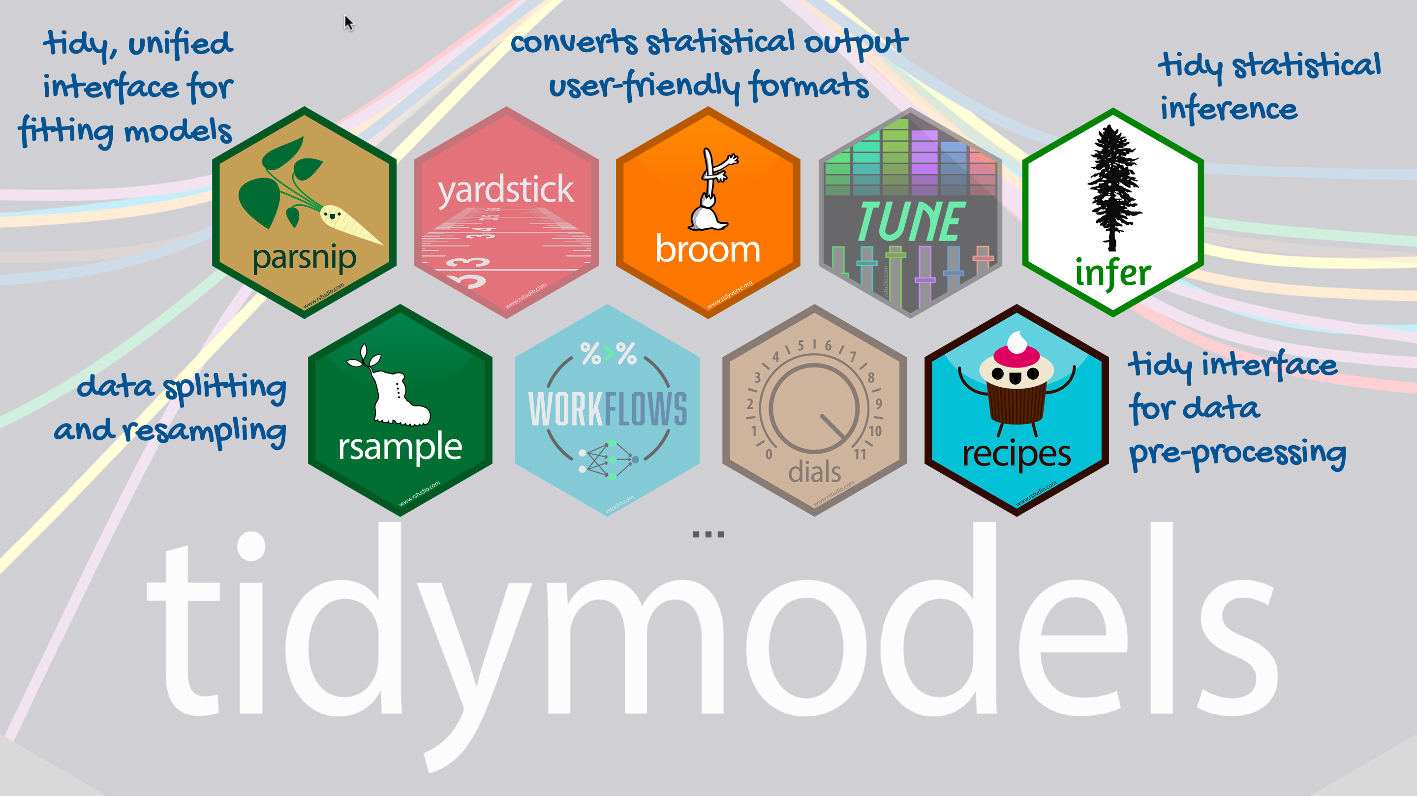
✔ broom        1.0.5     ✔ rsample      1.2.1
✔ dials        1.3.0     ✔ tune         1.2.1
✔ infer        1.0.7     ✔ workflows    1.1.4
✔ modeldata    1.3.0     ✔ workflowsets 1.1.0
✔ parsnip      1.2.1     ✔ yardstick    1.3.1
✔ recipes      1.1.0     
── Conflicts ───────────────────────────────────────── tidymodels_conflicts() ──
✖ scales::discard() masks purrr::discard()
✖ dplyr::filter()   masks stats::filter()
✖ recipes::fixed()  masks stringr::fixed()
✖ dplyr::lag()      masks stats::lag()
✖ yardstick::spec() masks readr::spec()
✖ recipes::step()   masks stats::step()
• Dig deeper into tidy modeling with R at https://www.tmwr.org

library(palmerpenguins)

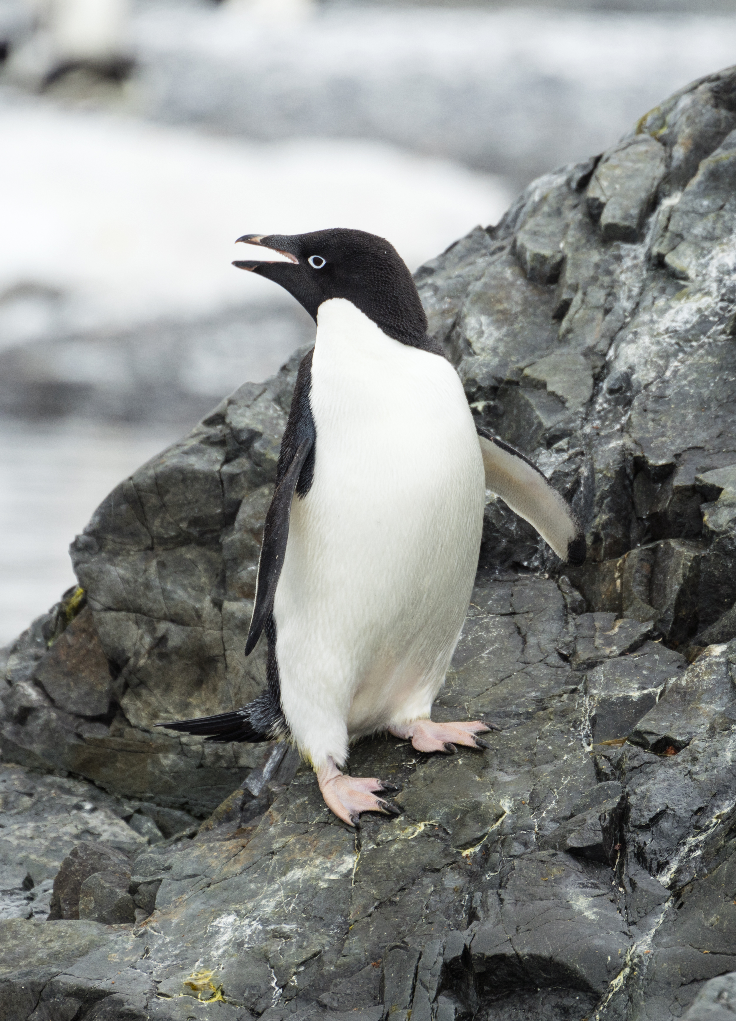
Attaching package: 'palmerpenguins'

The following object is masked from 'package:modeldata':

    penguins

Models in Science

What is a model?

• A model is an informative representation of an object, person or system.

• A model is a simplified representation of the real world focusing on the essential parts for its purpose.

Source: https://en.wikipedia.org/wiki/Model

Scientific Modeling

Scientific modeling is an activity that produces models representing empirical objects, phenomena, and physical processes, to make a particular part or feature of the world easier to

• understand,
• define,
• quantify,
• visualize, or
• simulate.

Famous wisdom

All models are wrong, but some are useful.

Source: https://en.wikipedia.org/wiki/Scientific_modelling

Model Purposes and Data Analysis

• Agent-based models and differential equations
  • are used to explain the dynamics of one or more variables (typically) over time. They are used to answer mechanistic questions.
• Variable-based models
  • are used to specify relations between variables
  • to explain relations and make predictions.
  • Used to answer inferential and predictive questions.
    
  • (With experimental and theoretical effort also for causal questions.)

The most basic variable-based model is the linear model.

Models to Learn from Data

In much of the following we use a narrower definition of model:

A mathematical model that consists of variables and functions.

Different names and roles of variables:

• random variables
• covariates
• predictors
• latent variables
• features
• targets
• outcomes

Functions relate variables to each other

• In a linear model we model one variable as a weighted sum of the other variables

Once a model (setup of variables and functions) is specified, modelers use Data to find the best function, called

• estimation
• training
• fitting
• learning

Modeling Mindsets

Even within the setup of Models to Learn from Data there are many different Modeling Mindsets

Molnar, C. (2022). Modeling mindsets: The many cultures of learning from data. Christoph Molnar c/o Mucbook Clubhouse.

Linear Model

The first work-horse model in data science

Hello again penguins!

We use the dataset Palmer Penguins

Chinstrap, Gentoo, and Adélie Penguins

penguins

# A tibble: 344 × 8
   species island    bill_length_mm bill_depth_mm flipper_length_mm body_mass_g
   <fct>   <fct>              <dbl>         <dbl>             <int>       <int>
 1 Adelie  Torgersen           39.1          18.7               181        3750
 2 Adelie  Torgersen           39.5          17.4               186        3800
 3 Adelie  Torgersen           40.3          18                 195        3250
 4 Adelie  Torgersen           NA            NA                  NA          NA
 5 Adelie  Torgersen           36.7          19.3               193        3450
 6 Adelie  Torgersen           39.3          20.6               190        3650
 7 Adelie  Torgersen           38.9          17.8               181        3625
 8 Adelie  Torgersen           39.2          19.6               195        4675
 9 Adelie  Torgersen           34.1          18.1               193        3475
10 Adelie  Torgersen           42            20.2               190        4250
# ℹ 334 more rows
# ℹ 2 more variables: sex <fct>, year <int>

Body mass in grams

penguins |>
  ggplot(aes(body_mass_g)) +
  geom_histogram()

`stat_bin()` using `bins = 30`. Pick better value with `binwidth`.

Warning: Removed 2 rows containing non-finite outside the scale range
(`stat_bin()`).

Flipper length in millimeters

penguins |>
  ggplot(aes(flipper_length_mm)) +
  geom_histogram()

`stat_bin()` using `bins = 30`. Pick better value with `binwidth`.

Warning: Removed 2 rows containing non-finite outside the scale range
(`stat_bin()`).

Relate variables as a line

A line is a shift-scale transformation of the identity function usually written in the form

\[f(x) = a\cdot x + b\]

where \(a\) is the slope, \(b\) is the intercept.¹

a <- 0.5
b <- 1
func <- function(x) a*x + b
ggplot() + geom_function(fun = func, size = 2) +
 # Set axis limits and make axis equal
    xlim(c(-0.5,2)) + ylim(c(0,2)) + coord_fixed() + 
    geom_line( # intercept line:
     data=tibble(x=c(0,0),y=c(0,1)), 
     mapping = aes(x,y), 
     color = "blue", size = 2) +
    geom_line( # slope:
     data=tibble(x=c(1.5,1.5),y=c(1.25,1.75)), 
     mapping = aes(x,y), 
     color = "red", size = 2) +
    geom_line( # x-interval of length one:
     data=tibble(x=c(0.5,1.5),y=c(1.25,1.25)), 
     mapping = aes(x,y), color = "gray") +
    theme_classic(base_size = 24)

Warning: Using `size` aesthetic for lines was deprecated in ggplot2 3.4.0.
ℹ Please use `linewidth` instead.

1. This a scale and a shift in the \(y\) direction. Note: For lines there is always an analog transformations on the \(x\) direction.

Penguins: Linear model

Flipper length as a function of body mass.

penguins |>
 ggplot(aes(x = body_mass_g, 
            y = flipper_length_mm)) +
 geom_point() +
 geom_smooth(method = "lm", 
             se = FALSE) + 
 theme_classic(base_size = 24)

`geom_smooth()` using formula = 'y ~ x'

Warning: Removed 2 rows containing non-finite outside the scale range
(`stat_smooth()`).

Warning: Removed 2 rows containing missing values or values outside the scale range
(`geom_point()`).

Penguins: A smooth line

Flipper length as a function of body mass with loess¹ smoothing.

penguins |>
 ggplot(aes(x = body_mass_g, 
            y = flipper_length_mm)) +
 geom_point() +
 geom_smooth(method = "loess") + 
 theme_classic(base_size = 24)

`geom_smooth()` using formula = 'y ~ x'

Warning: Removed 2 rows containing non-finite outside the scale range
(`stat_smooth()`).

Warning: Removed 2 rows containing missing values or values outside the scale range
(`geom_point()`).

This is a less theory-driven and more data-driven model. Why?
We don’t have a simple mathematical form of the function.

1. loess = locally estimated scatterplot smoothing

Terminology variable-based models

• Response variable:¹ Variable whose behavior or variation you are trying to understand, on the y-axis
• Explanatory variable(s):² Other variable(s) that you want to use to explain the variation in the response, on the x-axis
• Predicted value: Output of the model function.
  • The model function gives the (expected) average value of the response variable conditioning on the explanatory variables
  • Residual(s): A measure of how far away a case is from its predicted value (based on the particular model)
    Residual = Observed value minus Predicted value
    The residual tells how far above/below the expected value each case is

1. Also dependent variable in statistics or empirical social sciences.

2. Also independent variable(s) in statistics or empirical social sciences.

More explanatory variables

How does the relation between flipper length and body mass change with different species?

penguins |>
 ggplot(aes(x = body_mass_g, 
            y = flipper_length_mm, 
            color = species)) +
 geom_point() +
 geom_smooth(method = "lm",
             se = FALSE) + 
 theme_classic(base_size = 24)

`geom_smooth()` using formula = 'y ~ x'

Warning: Removed 2 rows containing non-finite outside the scale range
(`stat_smooth()`).

Warning: Removed 2 rows containing missing values or values outside the scale range
(`geom_point()`).

ggplot-hint: How to color penguins but keep one model?

Put the mapping of the color aesthetic into the geom_point command.

penguins |>
 ggplot(aes(x = body_mass_g, 
            y = flipper_length_mm)) +
 geom_point(aes(color = species)) +
 geom_smooth(method = "lm", se = FALSE) + 
 theme_classic(base_size = 24)

`geom_smooth()` using formula = 'y ~ x'

Warning: Removed 2 rows containing non-finite outside the scale range
(`stat_smooth()`).

Warning: Removed 2 rows containing missing values or values outside the scale range
(`geom_point()`).

Beware of Simpson’s paradox

Slopes for all groups can be in the opposite direction of the main effect’s slope!

Source: https://en.wikipedia.org/wiki/Simpson%27s_paradox

The paradox is real!

How does the relation between bill length and body mass change with different species?

penguins |>
 ggplot(aes(x = bill_length_mm, 
            y = bill_depth_mm)) +
 geom_point(aes(color = species)) +
 geom_smooth(mapping = aes(color = species),
             method = "lm",
             se = FALSE) + 
 geom_smooth(method = "lm",
                                                    se = FALSE) + 
 theme_classic(base_size = 24)

`geom_smooth()` using formula = 'y ~ x'

Warning: Removed 2 rows containing non-finite outside the scale range
(`stat_smooth()`).

`geom_smooth()` using formula = 'y ~ x'

Warning: Removed 2 rows containing non-finite outside the scale range
(`stat_smooth()`).

Warning: Removed 2 rows containing missing values or values outside the scale range
(`geom_point()`).

Models - upsides and downsides

• Models can reveal patterns that are not evident in a graph of the data. This is an advantage of modeling over simple visual inspection of data.
  • How would you visualize dependencies of more than two variables?
• The risk is that a model is imposing structure that is not really there in the real world data.
  • People imagined animal shapes in the stars. This is maybe a good model to detect and memorize shapes, but it has nothing to do with these animals.
  • Every model is a simplification of the real world, but there are good and bad models (for particular purposes).
  • A skeptical (but constructive) approach to a model is always advisable.

Variation around a model

… is as interesting and important as the model!

Statistics is the explanation of uncertainty of variation in the context of what remains unexplained.

• The scattered data of flipper length and body mass suggests that there maybe other factors that account for some parts of the variability.
• Or is it randomness?
• Adding more explanatory variables can help (but need not)

All models are wrong …

… but some are useful. (George Box)

Extending the range of the model:

penguins |>
 ggplot(aes(x = body_mass_g, 
            y = flipper_length_mm)) +
 geom_point() +
 geom_smooth(method = "lm", 
             se = FALSE, 
                                                fullrange = TRUE) +
    xlim(c(0,7000)) + ylim(c(0,230)) +
 theme_classic(base_size = 24)

`geom_smooth()` using formula = 'y ~ x'

Warning: Removed 3 rows containing non-finite outside the scale range
(`stat_smooth()`).

Warning: Removed 3 rows containing missing values or values outside the scale range
(`geom_point()`).

Warning: Removed 10 rows containing missing values or values outside the scale range
(`geom_smooth()`).

• The model predicts that penguins with zero weight still have flippers of about 140 mm on average.
• Is the model useless? Yes, around zero body mass. No, it works OK in the range of the body mass data.

Two model purposes

Linear models can be used for:

• Explanation: Understand the relationship of variables in a quantitative way.
  For the linear model, interpret slope and intercept.
  • In other words: We make inference about relations in any sample of penguins.
• Prediction: Plug in new values for the explanatory variable(s) and receive the expected response value.
  For the linear model, predict the flipper length of new penguins by their body mass.

Fitting Models

Today: The linear model.

In R: tidymodels

From https://datasciencebox.org

Our goal

Predict flipper length from body mass

average flipper_length_mm \(= \beta_0 + \beta_1\cdot\) body_mass_g

Step 1: Specify model

library(tidymodels)
linear_reg()

Linear Regression Model Specification (regression)

Computational engine: lm 

Step 2: Set the model fitting engine

linear_reg() |> 
    set_engine("lm")

Linear Regression Model Specification (regression)

Computational engine: lm 

Step 3: Fit model and estimate parameters

Only now, the data and the variable selection comes in.

Use of formula syntax

linear_reg() |> 
    set_engine("lm") |> 
    fit(flipper_length_mm ~ body_mass_g, data = penguins)

parsnip model object


Call:
stats::lm(formula = flipper_length_mm ~ body_mass_g, data = data)

Coefficients:
(Intercept)  body_mass_g  
  136.72956      0.01528  

parsnip is package in tidymodels which is to provide a tidy, unified interface to models that can be used to try a range of models.

Note: The fit command does not follow the tidyverse principle the data comes first. Instead, the formula comes first. This is to relate to existing traditions of a much older established way of modeling in base R.

What does the output say?

linear_reg() |> 
    set_engine("lm") |> 
    fit(flipper_length_mm ~ body_mass_g, data = penguins)

parsnip model object


Call:
stats::lm(formula = flipper_length_mm ~ body_mass_g, data = data)

Coefficients:
(Intercept)  body_mass_g  
  136.72956      0.01528  

average flipper_length_mm \(= 136.72956 + 0.01528\cdot\) body_mass_g

Interpretation:
The penguins have a flipper length of 138 mm plus 0.01528 mm for each gram of body mass (that is 15.28 mm per kg). Penguins with zero mass have a flipper length of 138 mm. However, this is not in the range where the model was fitted.

Show output in tidy form

linear_reg() |> 
    set_engine("lm") |> 
    fit(flipper_length_mm ~ body_mass_g, data = penguins) |> 
    tidy()

# A tibble: 2 × 5
  term        estimate std.error statistic   p.value
  <chr>          <dbl>     <dbl>     <dbl>     <dbl>
1 (Intercept) 137.      2.00          68.5 5.71e-201
2 body_mass_g   0.0153  0.000467      32.7 4.37e-107

Parameter estimation

Notation from statistics: \(\beta\)’s for the population parameters and \(\hat\beta\)’s for the parameters estimated from the sample statistics.

\[\hat y = \beta_0 + \beta_1 x\]

The population parameters \(\beta_0\) and \(\beta_1\) we cannot have.
\(\hat y\) stands for predicted value of \(y\).

Instead, we estimate \(\hat\beta_0\) and \(\hat\beta_1\) in the model fitting process.

\[\hat y = \hat\beta_0 + \hat\beta_1 x\]

A typical follow-up data analysis question is what the fitted values \(\hat\beta_0\) and \(\hat\beta_1\) tell us about the (unknown) population-wide values \(\beta_0\) and \(\beta_1\)?

This is the typical inferential question.

parsnip model objects

pengmod <- linear_reg() |> 
    set_engine("lm") |> 
    fit(flipper_length_mm ~ body_mass_g, data = penguins)
class(pengmod) # attributes

[1] "_lm"       "model_fit"

typeof(pengmod) 

[1] "list"

names(pengmod)

[1] "lvl"          "spec"         "fit"          "preproc"      "elapsed"     
[6] "censor_probs"

Most interesting for us for now: $fit

pengmod$fit

Call:
stats::lm(formula = flipper_length_mm ~ body_mass_g, data = data)

Coefficients:
(Intercept)  body_mass_g  
  136.72956      0.01528  

Notice: parsnip model object is now missing in the output.

$fit is the object created by lm (base R)

names(pengmod$fit)

 [1] "coefficients"  "residuals"     "effects"       "rank"         
 [5] "fitted.values" "assign"        "qr"            "df.residual"  
 [9] "na.action"     "xlevels"       "call"          "terms"        
[13] "model"        

pengmod$fit$call

stats::lm(formula = flipper_length_mm ~ body_mass_g, data = data)

pengmod$fit$coefficients

 (Intercept)  body_mass_g 
136.72955927   0.01527592 

pengmod$fit$fitted.values

       1        2        3        5        6        7        8        9 
194.0142 194.7780 186.3763 189.4315 192.4867 192.1048 208.1445 189.8134 
      10       11       12       13       14       15       16       17 
201.6522 187.1401 193.2504 185.6125 194.7780 203.9436 193.2504 189.4315 
      18       19       20       21       22       23       24       25 
205.4712 187.5220 200.8884 188.6677 191.7229 194.7780 197.0694 194.7780 
      26       27       28       29       30       31       32       33 
194.7780 190.9591 185.6125 184.8487 197.0694 186.3763 196.3056 187.1401 
      34       35       36       37       38       39       40       41 
196.3056 187.5220 200.1246 197.0694 190.9591 187.1401 207.7626 184.8487 
      42       43       44       45       46       47       48       49 
196.3056 184.0849 203.9436 182.5573 206.9988 189.0496 182.1754 189.4315 
      50       51       52       53       54       55       56       57 
200.1246 190.1953 202.4160 189.4315 198.5970 181.0297 193.2504 190.9591 
      58       59       60       61       62       63       64       65 
194.7780 180.2659 194.0142 184.8487 203.9436 191.7229 198.5970 180.2659 
      66       67       68       69       70       71       72       73 
197.0694 187.9039 199.3608 183.3211 204.7074 191.7229 196.3056 190.9591 
      74       75       76       77       78       79       80       81 
200.1246 193.2504 201.6522 193.2504 196.3056 190.9591 197.8332 185.6125 
      82       83       84       85       86       87       88       89 
208.5264 194.7780 200.8884 187.9039 190.9591 194.7780 190.1953 197.0694 
      90       91       92       93       94       95       96       97 
191.7229 190.9591 202.4160 188.6677 204.7074 187.1401 202.4160 193.2504 
      98       99      100      101      102      103      104      105 
203.1798 181.0297 199.3608 193.6323 208.9083 183.7030 201.6522 181.4116 
     106      107      108      109      110      111      112      113 
190.9591 194.0142 196.3056 185.2306 209.6721 195.1599 206.9988 185.6125 
     114      115      116      117      118      119      120      121 
202.0341 196.3056 198.9789 181.0297 194.3961 187.9039 187.5220 184.8487 
     122      123      124      125      126      127      128      129 
190.1953 189.4315 195.9237 183.3211 197.8332 186.7582 202.4160 183.3211 
     130      131      132      133      134      135      136      137 
197.8332 187.5220 190.1953 190.1953 205.0893 189.0496 196.3056 185.2306 
     138      139      140      141      142      143      144      145 
197.4513 188.6677 201.6522 188.6677 189.8134 183.3211 193.6323 182.5573 
     146      147      148      149      150      151      152      153 
192.4867 201.6522 189.8134 189.4315 194.0142 193.2504 197.8332 205.4712 
     154      155      156      157      158      159      160      161 
223.8023 204.7074 223.8023 219.2195 206.2350 210.0540 216.1643 203.9436 
     162      163      164      165      166      167      168      169 
215.4005 207.7626 221.5109 207.7626 226.0937 200.8884 226.0937 200.1246 
     170      171      172      173      174      175      176      177 
232.9678 210.0540 218.4557 223.8023 213.1091 203.9436 213.8729 213.1091 
     178      179      180      181      182      183      184      185 
214.6367 199.3608 223.0385 206.9988 221.5109 216.9281 208.5264 213.8729 
     186      187      188      189      190      191      192      193 
229.1488 215.4005 219.2195 212.3453 216.9281 203.1798 218.4557 197.0694 
     194      195      196      197      198      199      200      201 
223.8023 202.4160 209.2902 221.5109 211.5815 200.8884 219.2195 214.6367 
     202      203      204      205      206      207      208      209 
217.6919 210.8177 217.6919 203.9436 213.1091 211.5815 213.8729 202.4160 
     210      211      212      213      214      215      216      217 
213.1091 204.7074 221.5109 200.8884 217.6919 203.9436 223.0385 208.5264 
     218      219      220      221      222      223      224      225 
223.8023 207.7626 225.3299 208.5264 221.5109 209.2902 213.1091 214.6367 
     226      227      228      229      230      231      232      233 
216.1643 208.5264 225.3299 206.9988 228.3851 209.2902 227.6213 207.3807 
     234      235      236      237      238      239      240      241 
219.9833 208.9083 218.4557 209.2902 222.2747 206.9988 217.6919 211.1996 
     242      243      244      245      246      247      248      249 
221.5109 212.3453 219.2195 209.2902 223.0385 210.8177 216.1643 211.9634 
     250      251      252      253      254      255      256      257 
211.1996 207.3807 216.9281 210.8177 222.2747 212.7272 220.7471 208.9083 
     258      259      260      261      262      263      264      265 
220.7471 208.5264 220.7471 206.6169 220.7471 213.1091 227.6213 207.7626 
     266      267      268      269      270      271      273      274 
220.7471 203.5617 226.0937 211.1996 228.3851 211.9634 210.8177 224.5661 
     275      276      277      278      279      280      281      282 
216.1643 219.2195 190.1953 196.3056 192.4867 190.5772 193.6323 197.0694 
     283      284      285      286      287      288      289      290 
186.3763 194.0142 200.1246 193.2504 194.7780 194.3961 193.2504 198.5970 
     291      292      293      294      295      296      297      298 
191.3410 198.5970 187.1401 193.2504 189.4315 203.9436 191.7229 188.6677 
     299      300      301      302      303      304      305      306 
181.0297 194.7780 187.1401 200.1246 188.6677 194.7780 193.2504 206.2350 
     307      308      309      310      311      312      313      314 
185.6125 202.4160 187.9039 199.3608 191.7229 196.3056 195.5418 210.0540 
     315      316      317      318      319      320      321      322 
177.9745 205.4712 197.0694 192.4867 190.9591 190.1953 192.8685 204.7074 
     323      324      325      326      327      328      329      330 
188.6677 202.4160 186.3763 192.8685 187.5220 197.0694 191.7229 198.5970 
     331      332      333      334      335      336      337      338 
187.9039 189.4315 186.3763 198.5970 194.7780 190.5772 197.0694 192.4867 
     339      340      341      342      343      344 
192.4867 197.8332 188.6677 194.3961 199.3608 194.3961 

pengmod$fit$residuals

           1            2            3            5            6            7 
-13.01424280  -8.77803858   8.62371500   3.56853188  -2.48665124 -11.10475335 
           8            9           10           11           12           13 
-13.14446474   3.18663399 -11.65220061  -1.14008078 -13.25044702  -3.61248922 
          14           15           16           17           18           19 
 -3.77803858  -5.94358795  -8.25044702   5.56853188  -8.47117951  -3.52197867 
          20           21           22           23           24           25 
 -6.88840483 -14.66767234 -11.72285546  -5.77803858 -12.06942592 -14.77803858 
          26           27           28           29           30           31 
 -7.77803858  -7.95905968   1.38751078 -12.84869344 -17.06942592  -8.37628500 
          32           33           34           35           36           37 
-18.30563014   0.85991922 -12.30563014   7.47802133  -4.12460905  -7.06942592 
          38           39           40           41           42           43 
-10.95905968  -6.14008078 -23.76256685  -2.84869344  -1.30563014   1.91510234 
          44           45           46           47           48           49 
 -7.94358795   2.44269390 -16.99877107  -7.04957023  -3.17540821   0.56853188 
          50           51           52           53           54           55 
 -9.12460905  -4.19526390 -14.41599639   0.56853188   1.40298251   5.97028546 
          56           57           58           59           60           61 
 -2.25044702  -4.95905968  -1.77803858   0.73408124  -0.01424280   0.15130656 
          62           63           64           65           66           67 
 -8.94358795  -6.72285546  -6.59701749   3.73408124  -5.06942592   7.09612344 
          68           69           70           71           72           73 
-11.36081327   6.67889812  -6.70738373  -1.72285546  -6.30563014   5.04094032 
          74           75           76           77           78           79 
 -3.12460905  -3.25044702  -6.65220061  -2.25044702 -12.30563014  -3.95905968 
          80           81           82           83           84           85 
 -2.83322170   3.38751078 -12.52636263  -7.77803858  -7.88840483   3.09612344 
          86           87           88           89           90           91 
  3.04094032  -4.77803858  -1.19526390  -8.06942592  -1.72285546  11.04094032 
          92           93           94           95           96           97 
  2.58400361  -3.66767234 -18.70738373  -0.14008078   5.58400361  -3.25044702 
          98           99          100          101          102          103 
 -7.17979217  -3.02971454  -7.36081327  -1.63234491  -5.90826052  -0.70299977 
         104          105          106          107          108          109 
-11.65220061  11.58838757  -6.95905968   4.98575720  -6.30563014  -4.23059133 
         110          111          112          113          114          115 
-12.67205630   2.84006353 -15.99877107   7.38751078  -5.03409850  -5.30563014 
         116          117          118          119          120          121 
 -2.97891538   6.97028546   4.60385931   1.09612344   1.47802133   2.15130656 
         122          123          124          125          126          127 
  7.80473610 -13.43146812   6.07626775   2.67889812   1.16677830   4.24181711 
         128          129          130          131          132          133 
 -7.41599639   7.67889812  12.16677830   2.47802133   6.80473610   2.80473610 
         134          135          136          137          138          139 
 -6.08928162  -2.04957023  -6.30563014   5.76940867   2.54867619  -3.66767234 
         140          141          142          143          144          145 
 -8.65220061   4.33232766  -2.81336601   4.67889812  -3.63234491   9.44269390 
         146          147          148          149          150          151 
 -7.48665124 -11.65220061  -5.81336601   5.56853188  -1.01424280  -6.25044702 
         152          153          154          155          156          157 
  3.16677830   5.52882049   6.19772176   5.29261627  -5.80227824  -4.21950356 
         158          159          160          161          162          163 
  3.76502471   0.94604581   2.83567957   5.05641205  -0.40052465   6.23743315 
         164          165          166          167          168          169 
 -5.51089090   6.23743315 -13.09366558   9.11159517  -9.09366558   9.87539095 
         170          171          172          173          174          175 
-11.96782760  -1.05395419   3.54429222  -5.80227824   1.89086269   9.05641205 
         176          177          178          179          180          181 
  1.12706691   1.89086269   0.36327113  16.63918673  -8.03848246   3.00122893 
         182          183          184          185          186          187 
 -1.51089090   5.07188379   0.47363737  -6.87293309   0.85115130   4.59947535 
         188          189          190          191          192          193 
  0.78049644   0.65465847   2.07188379   4.82020783 -10.45570778  10.93057408 
         194          195          196          197          198          199 
  1.19772176   7.58400361   6.70984159   0.48910910   5.41845425   9.11159517 
         200          201          202          203          204          205 
  5.78049644  -1.63672887  -2.69191200  -0.81774997   2.30808800   6.05641205 
         206          207          208          209          210          211 
 11.89086269   5.41845425   6.12706691   5.58400361   6.89086269   3.29261627 
         212          213          214          215          216          217 
  2.48910910   7.11159517   3.30808800  10.05641205   7.96151754  10.47363737 
         218          219          220          221          222          223 
  6.19772176   6.23743315   3.67013020  11.47363737   1.48910910   6.70984159 
         224          225          226          227          228          229 
  7.89086269   6.36327113   0.83567957   7.47363737   4.67013020   2.00122893 
         230          231          232          233          234          235 
 -8.38505292   5.70984159  -4.62125714   4.61933104   1.01670066   3.09173948 
         236          237          238          239          240          241 
  5.54429222   2.70984159   5.72531332  11.00122893   0.30808800   0.80035214 
         242          243          244          245          246          247 
  8.48910910   5.65465847   8.78049644   2.70984159   0.96151754   3.18225003 
         248          249          250          251          252          253 
  9.83567957   4.03655636  10.80035214  -4.38066896   8.07188379   8.18225003 
         254          255          256          257          258          259 
  5.72531332   2.27276058   7.25290488   7.09173948  -5.74709512   1.47363737 
         260          261          262          263          264          265 
 -1.74709512   1.38312682 -11.74709512   2.89086269   1.37874286   5.23743315 
         266          267          268          269          270          271 
  9.25290488  13.43830994   3.90633442   5.80035214  -6.38505292   2.03655636 
         273          274          275          276          277          278 
  4.18225003  -2.56607402  -4.16432043  -6.21950356   1.80473610  -0.30563014 
         279          280          281          282          283          284 
  0.51334876  -2.57716179   3.36765509   0.93057408  -8.37628500   2.98575720 
         285          286          287          288          289          290 
 -5.12460905   4.74955298  -1.77803858  -0.39614069  -8.25044702   2.40298251 
         291          292          293          294          295          296 
 -1.34095757   2.40298251   9.85991922 -12.25044702   0.56853188  -8.94358795 
         297          298          299          300          301          302 
-10.72285546   2.33232766   5.97028546  -1.77803858   7.85991922  -3.12460905 
         303          304          305          306          307          308 
 11.33232766   5.22196142  -2.25044702  -1.23497529   1.38751078  -1.41599639 
         309          310          311          312          313          314 
 -0.90387656   3.63918673   3.27714454   2.69436986  -0.54183436  -0.05395419 
         315          316          317          318          319          320 
 14.02546859  -0.47117951  12.93057408  -5.48665124   5.04094032   5.80473610 
         321          322          323          324          325          326 
  3.13145087  -3.70738373   1.33232766   9.58400361   0.62371500   5.13145087 
         327          328          329          330          331          332 
 11.47802133   3.93057408   1.27714454   4.40298251  -0.90387656   7.56853188 
         333          334          335          336          337          338 
  4.62371500   4.40298251   7.22196142   3.42283821   8.93057408  -3.48665124 
         339          340          341          342          343          344 
  2.51334876   9.16677830  13.33232766  -1.39614069  10.63918673   3.60385931 

Fitting method: Least squares regression

• The regression line shall minimize the sum of the squared residuals
  (or, identically, their mean).
• Mathematically: The residual for case \(i\) is \(e_i = \hat y_i - y_i\).
• Now we want to minimize \(\sum_{i=1}^n e_i^2\)
  (or equivalently \(\frac{1}{n}\sum_{i=1}^n e_i^2\) the mean of squared errors, which we will look at later).

Visualization of residuals

The residuals are the gray lines between predicted values on the regression line and the actual values.

pengmod <- 
  linear_reg() |> 
  set_engine("lm") |> 
  fit(flipper_length_mm ~ body_mass_g, data = penguins)
penguins |> bind_cols(predict(pengmod,penguins)) |> 
  ggplot(aes(body_mass_g, flipper_length_mm)) +
  geom_segment(aes(x = body_mass_g, y = flipper_length_mm, xend = body_mass_g, yend = .pred), color = "gray") +
  geom_point(alpha = 0.3) +
  geom_smooth(method="lm") + 
  geom_point(aes(y=.pred), color = "red", alpha =  0.3)

`geom_smooth()` using formula = 'y ~ x'

Warning: Removed 2 rows containing non-finite outside the scale range
(`stat_smooth()`).

Warning: Removed 2 rows containing missing values or values outside the scale range
(`geom_segment()`).

Warning: Removed 2 rows containing missing values or values outside the scale range
(`geom_point()`).
Removed 2 rows containing missing values or values outside the scale range
(`geom_point()`).

Check: Fitted values and Residuals

Recall: Residual = Observed value - Predicted value

The Predicted values are also called Fitted values. Hence:

Residuals + Fitted values = Observed values

pengmod$fit$residuals + pengmod$fit$fitted.values

  1   2   3   5   6   7   8   9  10  11  12  13  14  15  16  17  18  19  20  21 
181 186 195 193 190 181 195 193 190 186 180 182 191 198 185 195 197 184 194 174 
 22  23  24  25  26  27  28  29  30  31  32  33  34  35  36  37  38  39  40  41 
180 189 185 180 187 183 187 172 180 178 178 188 184 195 196 190 180 181 184 182 
 42  43  44  45  46  47  48  49  50  51  52  53  54  55  56  57  58  59  60  61 
195 186 196 185 190 182 179 190 191 186 188 190 200 187 191 186 193 181 194 185 
 62  63  64  65  66  67  68  69  70  71  72  73  74  75  76  77  78  79  80  81 
195 185 192 184 192 195 188 190 198 190 190 196 197 190 195 191 184 187 195 189 
 82  83  84  85  86  87  88  89  90  91  92  93  94  95  96  97  98  99 100 101 
196 187 193 191 194 190 189 189 190 202 205 185 186 187 208 190 196 178 192 192 
102 103 104 105 106 107 108 109 110 111 112 113 114 115 116 117 118 119 120 121 
203 183 190 193 184 199 190 181 197 198 191 193 197 191 196 188 199 189 189 187 
122 123 124 125 126 127 128 129 130 131 132 133 134 135 136 137 138 139 140 141 
198 176 202 186 199 191 195 191 210 190 197 193 199 187 190 191 200 185 193 193 
142 143 144 145 146 147 148 149 150 151 152 153 154 155 156 157 158 159 160 161 
187 188 190 192 185 190 184 195 193 187 201 211 230 210 218 215 210 211 219 209 
162 163 164 165 166 167 168 169 170 171 172 173 174 175 176 177 178 179 180 181 
215 214 216 214 213 210 217 210 221 209 222 218 215 213 215 215 215 216 215 210 
182 183 184 185 186 187 188 189 190 191 192 193 194 195 196 197 198 199 200 201 
220 222 209 207 230 220 220 213 219 208 208 208 225 210 216 222 217 210 225 213 
202 203 204 205 206 207 208 209 210 211 212 213 214 215 216 217 218 219 220 221 
215 210 220 210 225 217 220 208 220 208 224 208 221 214 231 219 230 214 229 220 
222 223 224 225 226 227 228 229 230 231 232 233 234 235 236 237 238 239 240 241 
223 216 221 221 217 216 230 209 220 215 223 212 221 212 224 212 228 218 218 212 
242 243 244 245 246 247 248 249 250 251 252 253 254 255 256 257 258 259 260 261 
230 218 228 212 224 214 226 216 222 203 225 219 228 215 228 216 215 210 219 208 
262 263 264 265 266 267 268 269 270 271 273 274 275 276 277 278 279 280 281 282 
209 216 229 213 230 217 230 217 222 214 215 222 212 213 192 196 193 188 197 198 
283 284 285 286 287 288 289 290 291 292 293 294 295 296 297 298 299 300 301 302 
178 197 195 198 193 194 185 201 190 201 197 181 190 195 181 191 187 193 195 197 
303 304 305 306 307 308 309 310 311 312 313 314 315 316 317 318 319 320 321 322 
200 200 191 205 187 201 187 203 195 199 195 210 192 205 210 187 196 196 196 201 
323 324 325 326 327 328 329 330 331 332 333 334 335 336 337 338 339 340 341 342 
190 212 187 198 199 201 193 203 187 197 191 203 202 194 206 189 195 207 202 193 
343 344 
210 198 

penguins$flipper_length_mm

  [1] 181 186 195  NA 193 190 181 195 193 190 186 180 182 191 198 185 195 197
 [19] 184 194 174 180 189 185 180 187 183 187 172 180 178 178 188 184 195 196
 [37] 190 180 181 184 182 195 186 196 185 190 182 179 190 191 186 188 190 200
 [55] 187 191 186 193 181 194 185 195 185 192 184 192 195 188 190 198 190 190
 [73] 196 197 190 195 191 184 187 195 189 196 187 193 191 194 190 189 189 190
 [91] 202 205 185 186 187 208 190 196 178 192 192 203 183 190 193 184 199 190
[109] 181 197 198 191 193 197 191 196 188 199 189 189 187 198 176 202 186 199
[127] 191 195 191 210 190 197 193 199 187 190 191 200 185 193 193 187 188 190
[145] 192 185 190 184 195 193 187 201 211 230 210 218 215 210 211 219 209 215
[163] 214 216 214 213 210 217 210 221 209 222 218 215 213 215 215 215 216 215
[181] 210 220 222 209 207 230 220 220 213 219 208 208 208 225 210 216 222 217
[199] 210 225 213 215 210 220 210 225 217 220 208 220 208 224 208 221 214 231
[217] 219 230 214 229 220 223 216 221 221 217 216 230 209 220 215 223 212 221
[235] 212 224 212 228 218 218 212 230 218 228 212 224 214 226 216 222 203 225
[253] 219 228 215 228 216 215 210 219 208 209 216 229 213 230 217 230 217 222
[271] 214  NA 215 222 212 213 192 196 193 188 197 198 178 197 195 198 193 194
[289] 185 201 190 201 197 181 190 195 181 191 187 193 195 197 200 200 191 205
[307] 187 201 187 203 195 199 195 210 192 205 210 187 196 196 196 201 190 212
[325] 187 198 199 201 193 203 187 197 191 203 202 194 206 189 195 207 202 193
[343] 210 198

Proporties of least squares regression

The regression lines goes through the point (mean(x), mean(y)).

mean(penguins$body_mass_g, na.rm = TRUE)

[1] 4201.754

mean(penguins$flipper_length_mm, na.rm = TRUE)

[1] 200.9152

penguins |> bind_cols(predict(pengmod,penguins)) |> 
  ggplot(aes(body_mass_g, flipper_length_mm)) +
  geom_segment(aes(x = body_mass_g, y = flipper_length_mm, xend = body_mass_g, yend = .pred), color = "gray") +
  geom_point(alpha = 0.3) +
  geom_smooth(method="lm") + 
  geom_point(aes(y=.pred), color = "red", alpha =  0.3) + 
  geom_point(data = tibble(x = mean(penguins$body_mass_g, na.rm = T), y = mean(penguins$flipper_length_mm, na.rm = T)), 
                                            mapping = aes(x,y), color = "green", size = 5)

`geom_smooth()` using formula = 'y ~ x'

Warning: Removed 2 rows containing non-finite outside the scale range
(`stat_smooth()`).

Warning: Removed 2 rows containing missing values or values outside the scale range
(`geom_segment()`).

Warning: Removed 2 rows containing missing values or values outside the scale range
(`geom_point()`).
Removed 2 rows containing missing values or values outside the scale range
(`geom_point()`).

Proporties of least squares regression

Residuals sum up to zero

pengmod <- linear_reg() |>  set_engine("lm") |> fit(flipper_length_mm ~ body_mass_g, data = penguins)
pengmod$fit$residuals |> sum()

[1] -1.135758e-13

There is no correlation between residuals and the explanatory variable

cor(pengmod$fit$residuals, na.omit(penguins$body_mass_g))

[1] -1.083343e-16

The correlation of \(x\) and \(y\) is the slope \(\beta_1\) “corrected” by their standard deviations.

correlation <- cor(penguins$flipper_length_mm, penguins$body_mass_g, use = "pairwise.complete.obs")
sd_flipper <- sd(penguins$flipper_length_mm, na.rm = T)
sd_mass <- sd(penguins$body_mass_g, na.rm = T)
c(correlation, sd_flipper, sd_mass)

[1]   0.8712018  14.0617137 801.9545357

correlation * sd_flipper / sd_mass

[1] 0.01527592

pengmod$fit$coefficients

 (Intercept)  body_mass_g 
136.72955927   0.01527592 

Correlation and linear regression

When the two variables in the linear regression are standardized (standard scores)

• the intercept is zero
• the coefficient coincides with the correlation

Linear Models and Dummy Variables

Explanatory variables are categorical

Let’s try what happens with species as explanatory variable. Remember, we have three species: Adelie, Chinstrap, Gentoo.

linear_reg() |> 
    set_engine("lm") |> 
    fit(flipper_length_mm ~ species, data = penguins) |> 
    tidy()

# A tibble: 3 × 5
  term             estimate std.error statistic   p.value
  <chr>               <dbl>     <dbl>     <dbl>     <dbl>
1 (Intercept)        190.       0.540    351.   0        
2 speciesChinstrap     5.87     0.970      6.05 3.79e-  9
3 speciesGentoo       27.2      0.807     33.8  1.84e-110

What happened?

Two of the three species categories appear as variables now.

• Categorical variables are automatically encoded to dummy variables
• Each coefficient describes the expected difference between flipper length of that particular species compared to the baseline level
• What is the baseline level? The first category! (Here alphabetically "Adelie")

How do dummy variables look?

species	speciesChinstrap	speciesGentoo
Adelie	0	0
Adelie	0	0
Chinstrap	1	0
Gentoo	0	1
Gentoo	0	1
Gentoo	0	1
Adelie	0	0
Chinstrap	1	0

Then the fitting of the linear model is as before using the zero-one variables.

Interpretation

linear_reg() |> 
    set_engine("lm") |> 
    fit(flipper_length_mm ~ species, data = penguins) |> 
    tidy()

# A tibble: 3 × 5
  term             estimate std.error statistic   p.value
  <chr>               <dbl>     <dbl>     <dbl>     <dbl>
1 (Intercept)        190.       0.540    351.   0        
2 speciesChinstrap     5.87     0.970      6.05 3.79e-  9
3 speciesGentoo       27.2      0.807     33.8  1.84e-110

• Flipper length of the baseline species is the intercept.
  • Average flipper length of Adelie is 190 mm
• Flipper length of the two other species add their coefficient
  • Average flipper length of Chinstrap is 190 + 5.87 mm
  • Average flipper length of Gentoo is 190 + 27.2 mm

Compare to a visualization

linear_reg() |> 
    set_engine("lm") |> 
    fit(flipper_length_mm ~ species, data = penguins) |> 
    tidy()

# A tibble: 3 × 5
  term             estimate std.error statistic   p.value
  <chr>               <dbl>     <dbl>     <dbl>     <dbl>
1 (Intercept)        190.       0.540    351.   0        
2 speciesChinstrap     5.87     0.970      6.05 3.79e-  9
3 speciesGentoo       27.2      0.807     33.8  1.84e-110

penguins |> 
  ggplot(aes(species, flipper_length_mm)) + geom_boxplot() +
    stat_summary(fun.y=mean, geom="point", size=5, color="red")

Warning: The `fun.y` argument of `stat_summary()` is deprecated as of ggplot2 3.3.0.
ℹ Please use the `fun` argument instead.

Warning: Removed 2 rows containing non-finite outside the scale range
(`stat_boxplot()`).

Warning: Removed 2 rows containing non-finite outside the scale range
(`stat_summary()`).

The red dots are the average values for species.

Linear models and R-squared

Quality of different linear models?

linear_reg() |> set_engine("lm") |> 
    fit(flipper_length_mm ~ body_mass_g, data = penguins) |> 
 tidy()

# A tibble: 2 × 5
  term        estimate std.error statistic   p.value
  <chr>          <dbl>     <dbl>     <dbl>     <dbl>
1 (Intercept) 137.      2.00          68.5 5.71e-201
2 body_mass_g   0.0153  0.000467      32.7 4.37e-107

average flipper_length_mm \(= 137 + 0.0153\cdot\) body_mass_g

linear_reg() |> set_engine("lm") |> 
    fit(bill_depth_mm ~ bill_length_mm, data = penguins) |> 
 tidy()

# A tibble: 2 × 5
  term           estimate std.error statistic  p.value
  <chr>             <dbl>     <dbl>     <dbl>    <dbl>
1 (Intercept)     20.9       0.844      24.7  4.72e-78
2 bill_length_mm  -0.0850    0.0191     -4.46 1.12e- 5

average bill_depth_mm \(= 20.9 -0.085\cdot\) bill_length_mm

Technical: The idea of the tidy() function is to turn an object into a tidy tibble. Here, it extracts the coefficients of the linear model (and more statistical information).

R-squared of a fitted model

\(R^2\) is the percentage of variability in the response explained by the regression model.

R-squared is also called coefficient of determination.

Definition:

\(R^2 = 1 - \frac{SS_\text{res}}{SS_\text{tot}}\)

where \(SS_\text{res} = \sum_i(y_i - f_i)^2 = \sum_i e_i^2\) is the sum of the squared residuals, and
\(SS_\text{tot} = \sum_i(y_i - \bar y)^2\) the total sum of squares which is proportional to the variance of \(y\). (\(\bar y\) is the mean of \(y\).)

Linear model R-squared

linear_reg() |> set_engine("lm") |> 
 fit(flipper_length_mm ~ body_mass_g, data = penguins) |>
 glance()  # glance shows summary statistics of model fit

# A tibble: 1 × 12
  r.squared adj.r.squared sigma statistic   p.value    df logLik   AIC   BIC
      <dbl>         <dbl> <dbl>     <dbl>     <dbl> <dbl>  <dbl> <dbl> <dbl>
1     0.759         0.758  6.91     1071. 4.37e-107     1 -1146. 2297. 2309.
# ℹ 3 more variables: deviance <dbl>, df.residual <int>, nobs <int>

Interpretation R-squared? 75.9% of the variance of flipper length can be explained by a linear relation with body mass.

linear_reg() |> set_engine("lm") |> 
    fit(bill_depth_mm ~ bill_length_mm, data = penguins) |> 
 glance()

# A tibble: 1 × 12
  r.squared adj.r.squared sigma statistic   p.value    df logLik   AIC   BIC
      <dbl>         <dbl> <dbl>     <dbl>     <dbl> <dbl>  <dbl> <dbl> <dbl>
1    0.0552        0.0525  1.92      19.9 0.0000112     1  -708. 1422. 1433.
# ℹ 3 more variables: deviance <dbl>, df.residual <int>, nobs <int>

5.52% of the variance of bill depth can be explained by a linear relation with bill length.

Technical: The idea of the glance() function is to construct a single row summary “glance” of a model, fit, or other object.

R-squared and correlation

For a linear model with one predictor, the square of the correlation coefficient is the same as the R-squared of the model.

linear_reg() |> set_engine("lm") |> 
    fit(flipper_length_mm ~ body_mass_g, data = penguins) |> 
 glance()

# A tibble: 1 × 12
  r.squared adj.r.squared sigma statistic   p.value    df logLik   AIC   BIC
      <dbl>         <dbl> <dbl>     <dbl>     <dbl> <dbl>  <dbl> <dbl> <dbl>
1     0.759         0.758  6.91     1071. 4.37e-107     1 -1146. 2297. 2309.
# ℹ 3 more variables: deviance <dbl>, df.residual <int>, nobs <int>

cor(penguins$flipper_length_mm, penguins$body_mass_g, use = "pairwise.complete.obs")

[1] 0.8712018

cor(penguins$flipper_length_mm, penguins$body_mass_g, use = "pairwise.complete.obs")^2

[1] 0.7589925

Hence, the name \(R^2\)!

Linear models with more predictors

More predictors: Coefficients

linear_reg() |> set_engine("lm") |> 
 fit(flipper_length_mm ~ body_mass_g, data = penguins) |> 
 tidy()

# A tibble: 2 × 5
  term        estimate std.error statistic   p.value
  <chr>          <dbl>     <dbl>     <dbl>     <dbl>
1 (Intercept) 137.      2.00          68.5 5.71e-201
2 body_mass_g   0.0153  0.000467      32.7 4.37e-107

linear_reg() |> set_engine("lm") |> 
 fit(flipper_length_mm ~ body_mass_g + bill_length_mm, data = penguins) |> 
 tidy()

# A tibble: 3 × 5
  term           estimate std.error statistic   p.value
  <chr>             <dbl>     <dbl>     <dbl>     <dbl>
1 (Intercept)    122.      2.86         42.7  1.70e-138
2 body_mass_g      0.0131  0.000545     23.9  7.56e- 75
3 bill_length_mm   0.549   0.0801        6.86 3.31e- 11

linear_reg() |> set_engine("lm") |> 
 fit(flipper_length_mm ~ body_mass_g + bill_length_mm + bill_depth_mm, data = penguins) |> 
 tidy()

# A tibble: 4 × 5
  term           estimate std.error statistic   p.value
  <chr>             <dbl>     <dbl>     <dbl>     <dbl>
1 (Intercept)    158.      4.63         34.1  1.80e-111
2 body_mass_g      0.0109  0.000538     20.3  1.93e- 60
3 bill_length_mm   0.592   0.0717        8.26 3.42e- 15
4 bill_depth_mm   -1.68    0.181        -9.29 1.99e- 18

More predictors: glance R-squared

linear_reg() |> set_engine("lm") |> 
 fit(flipper_length_mm ~ body_mass_g, data = penguins) |> 
 glance()

# A tibble: 1 × 12
  r.squared adj.r.squared sigma statistic   p.value    df logLik   AIC   BIC
      <dbl>         <dbl> <dbl>     <dbl>     <dbl> <dbl>  <dbl> <dbl> <dbl>
1     0.759         0.758  6.91     1071. 4.37e-107     1 -1146. 2297. 2309.
# ℹ 3 more variables: deviance <dbl>, df.residual <int>, nobs <int>

linear_reg() |> set_engine("lm") |> 
 fit(flipper_length_mm ~ body_mass_g + bill_length_mm, data = penguins) |> 
 glance()

# A tibble: 1 × 12
  r.squared adj.r.squared sigma statistic   p.value    df logLik   AIC   BIC
      <dbl>         <dbl> <dbl>     <dbl>     <dbl> <dbl>  <dbl> <dbl> <dbl>
1     0.788         0.787  6.49      631. 4.88e-115     2 -1123. 2255. 2270.
# ℹ 3 more variables: deviance <dbl>, df.residual <int>, nobs <int>

linear_reg() |> set_engine("lm") |> 
 fit(flipper_length_mm ~ body_mass_g + bill_length_mm + bill_depth_mm, data = penguins) |> 
 glance()

# A tibble: 1 × 12
  r.squared adj.r.squared sigma statistic   p.value    df logLik   AIC   BIC
      <dbl>         <dbl> <dbl>     <dbl>     <dbl> <dbl>  <dbl> <dbl> <dbl>
1     0.831         0.830  5.80      556. 2.99e-130     3 -1084. 2179. 2198.
# ℹ 3 more variables: deviance <dbl>, df.residual <int>, nobs <int>

More predictors: Equations

average flipper_length_mm \(= 137 + 0.0153\cdot\) body_mass_g
75.9% explained variance

average flipper_length_mm \(= 122 + 0.0131\cdot\) body_mass_g \(+ 0.549\cdot\) bill_length_mm
78.8% explained variance

average flipper_length_mm \(= 158 + 0.0109\cdot\) body_mass_g \(+ 0.592\cdot\) bill_length_mm \(+ 1.68\cdot\) bill_length_mm
83.1% explained variance

Interaction Effects

Adding products of variables as new variable.

Adding a categorical variable as main effect

linear_reg() |> set_engine("lm") |> 
 fit(flipper_length_mm ~ body_mass_g + species, data = penguins) |> 
 tidy()

# A tibble: 4 × 5
  term              estimate std.error statistic   p.value
  <chr>                <dbl>     <dbl>     <dbl>     <dbl>
1 (Intercept)      159.       2.39         66.6  2.45e-196
2 body_mass_g        0.00840  0.000634     13.3  1.40e- 32
3 speciesChinstrap   5.60     0.788         7.10 7.33e- 12
4 speciesGentoo     15.7      1.09         14.4  6.80e- 37

A main effect by categorical dummy variables allows for different intercepts per species. (However, the slopes are the same.)

linear_reg() |> set_engine("lm") |> 
 fit(flipper_length_mm ~ body_mass_g + species, data = penguins) |> 
 glance()

# A tibble: 1 × 12
  r.squared adj.r.squared sigma statistic   p.value    df logLik   AIC   BIC
      <dbl>         <dbl> <dbl>     <dbl>     <dbl> <dbl>  <dbl> <dbl> <dbl>
1     0.854         0.853  5.40      659. 7.42e-141     3 -1060. 2129. 2149.
# ℹ 3 more variables: deviance <dbl>, df.residual <int>, nobs <int>

Adding species increases R-squared better than adding bill length and bill depth together!

Adding as interaction effect

linear_reg() |> set_engine("lm") |> 
 fit(flipper_length_mm ~ body_mass_g * species, data = penguins) |> 
 tidy()

# A tibble: 6 × 5
  term                          estimate std.error statistic   p.value
  <chr>                            <dbl>     <dbl>     <dbl>     <dbl>
1 (Intercept)                  165.       3.55         46.5  1.56e-148
2 body_mass_g                    0.00668  0.000952      7.01 1.30e- 11
3 speciesChinstrap             -13.9      7.30         -1.90 5.84e-  2
4 speciesGentoo                  6.06     6.05          1.00 3.17e-  1
5 body_mass_g:speciesChinstrap   0.00523  0.00195       2.68 7.66e-  3
6 body_mass_g:speciesGentoo      0.00236  0.00135       1.75 8.16e-  2

• Note the * for interaction effect!
• Also main effects for both variables are in as coefficients.
• Adelie is the baseline species (because it is first in the alphabet).
• An interaction effect allows for different slopes for each species!

Regression lines by species

penguins |> 
  ggplot(aes(x = body_mass_g, y = flipper_length_mm, color = species)) +
  geom_point() + geom_smooth(method = "lm") +
  theme_minimal()

`geom_smooth()` using formula = 'y ~ x'

Warning: Removed 2 rows containing non-finite outside the scale range
(`stat_smooth()`).

Warning: Removed 2 rows containing missing values or values outside the scale range
(`geom_point()`).

Compare the slopes to the regression output on the slides before!

Different equations for each species!

linear_reg() |> set_engine("lm") |> 
 fit(flipper_length_mm ~ body_mass_g * species, data = penguins) |> 
 tidy()

# A tibble: 6 × 5
  term                          estimate std.error statistic   p.value
  <chr>                            <dbl>     <dbl>     <dbl>     <dbl>
1 (Intercept)                  165.       3.55         46.5  1.56e-148
2 body_mass_g                    0.00668  0.000952      7.01 1.30e- 11
3 speciesChinstrap             -13.9      7.30         -1.90 5.84e-  2
4 speciesGentoo                  6.06     6.05          1.00 3.17e-  1
5 body_mass_g:speciesChinstrap   0.00523  0.00195       2.68 7.66e-  3
6 body_mass_g:speciesGentoo      0.00236  0.00135       1.75 8.16e-  2

Adelie:
average flipper_length_mm \(= 165 + 0.00668\cdot\) body_mass_g

Chinstrap:
average flipper_length_mm \(= 165 - 13.6 + (0.00668 + 0.00523)\cdot\) body_mass_g

Gentoo:
average flipper_length_mm \(= 165 + 6.06 + (0.00668 + 0.00236)\cdot\) body_mass_g

Improvement of interaction effects is small here

linear_reg() |> set_engine("lm") |> 
 fit(flipper_length_mm ~ body_mass_g + species, data = penguins) |> 
 glance()

# A tibble: 1 × 12
  r.squared adj.r.squared sigma statistic   p.value    df logLik   AIC   BIC
      <dbl>         <dbl> <dbl>     <dbl>     <dbl> <dbl>  <dbl> <dbl> <dbl>
1     0.854         0.853  5.40      659. 7.42e-141     3 -1060. 2129. 2149.
# ℹ 3 more variables: deviance <dbl>, df.residual <int>, nobs <int>

linear_reg() |> set_engine("lm") |> 
 fit(flipper_length_mm ~ body_mass_g * species, data = penguins) |> 
 glance()

# A tibble: 1 × 12
  r.squared adj.r.squared sigma statistic   p.value    df logLik   AIC   BIC
      <dbl>         <dbl> <dbl>     <dbl>     <dbl> <dbl>  <dbl> <dbl> <dbl>
1     0.857         0.855  5.35      404. 9.60e-140     5 -1056. 2125. 2152.
# ℹ 3 more variables: deviance <dbl>, df.residual <int>, nobs <int>

Interaction effects of two categoricals

Assume \(x_1\) and \(x_2\) are categorical variables. We add their product in the linear model as a new variable: \(y_i = \beta_0 + \beta_1x_1 + \beta_2x_2 + \beta_{3}x_1x_2 + \dots\).

Example: \(x_1\) is gender female and \(x_2\) having kids

tibble(gender_female = c(0,1,1,0), has_kids = c(1,0,1,0)) |> 
 mutate(gender_female_x_has_kids = gender_female * has_kids) |> 
 knitr::kable()

gender_female	has_kids	gender_female_x_has_kids
0	1	0
1	0	0
1	1	1
0	0	0

• What is the baseline? Being male without kids.
• Thought experiment: When we estimate a model explaining life satisfaction with these. How would we see if being a mother increases life satisfaction more than being a father? positive coefficient for gender_female_x_has_kids

Nonlinear Models

When a linear model is bad

Example: Total corona cases in Germany in the first wave 2020.

whofull <- read_csv("data/WHO-COVID-19-global-data.csv", show_col_types = FALSE) |> 
    filter(Country == "Germany") 
who <- whofull |> 
    filter(Date_reported < "2020-03-20", Date_reported > "2020-02-25") 
who |> 
    ggplot(aes(Date_reported, Cumulative_cases)) + 
    geom_line() + geom_point() + geom_smooth(method = "lm")

`geom_smooth()` using formula = 'y ~ x'

\(\log\) transformation

Instead of Cumulative_cases we look at \(\log(\)Cumulative_cases\()\)

    who |> 
    ggplot(aes(Date_reported, log(Cumulative_cases))) + geom_line() + geom_point() +
    geom_smooth(method = "lm") + theme_minimal(base_size = 20)

`geom_smooth()` using formula = 'y ~ x'

Almost perfect fit of the linear model: \(\log(y)=\log(\beta_0) + \beta_1\cdot x\)
(\(y=\) Cumulative cases, \(x=\) Days)

Exponentiation gives the model: \(y=\beta_0 e^{\beta_1\cdot x}\)
(Check \(e^{\log(\beta_0) + \beta_1\cdot x} = e^{\log(\beta_0)} e^{\beta_1\cdot x} = \beta_0 e^{\beta_1\cdot x}\))

Exponential growth!

\(y=\beta_0 e^{\beta_1\cdot x}\)
For comparison: Logistic function \(y = \frac{N \beta_0 e^{\beta_1\cdot x}}{N + \beta_0 e^{\beta_1\cdot x}}\) for \(N=200000\)

wholm <-    who |> 
 lm(log(Cumulative_cases) ~ Date_reported, data = _) 
who |> 
    ggplot(aes(Date_reported, Cumulative_cases)) + geom_line() + geom_point() +
 geom_function(fun = function(x) exp(coef(wholm)[1] + coef(wholm)[2]*as.numeric(x)), color = "red") + 
 geom_function(
  fun = function(x) 200000*exp(coef(wholm)[1] + coef(wholm)[2]*as.numeric(x))/(200000 + exp(coef(wholm)[1] + coef(wholm)[2]*as.numeric(x))), color = "blue") +
 theme_minimal(base_size = 20)

Logistic growth (as in the SI model) mimicks exponential growth initially.

\(\log\) transformation

    who |> 
    ggplot(aes(Date_reported, log10(Cumulative_cases))) + geom_line() + geom_point() +
    geom_smooth(method = "lm") 

`geom_smooth()` using formula = 'y ~ x'

An important difference of log10(Cumulative_cases) ~ Date_Reported to the penguin model flipper_length_mm ~ body_mass_g? ?

• \(x\) has an ordered structure and no duplicates

The fit looks so good. Why?

Because there is a mechanistic explanation behind: The SI model.

However, it works only in a certain range

who |> 
    ggplot(aes(Date_reported, Cumulative_cases)) + geom_point() +
 geom_function(fun = function(x) exp(coef(wholm)[1] + coef(wholm)[2]*as.numeric(x)), color = "red") + 
 geom_function(
  fun = function(x) 200000*exp(coef(wholm)[1] + coef(wholm)[2]*as.numeric(x))/(200000 + exp(coef(wholm)[1] + coef(wholm)[2]*as.numeric(x))), color = "blue") +
 theme_minimal(base_size = 20) +
 geom_line(data = whofull |> filter(Date_reported < "2020-06-30")) + ylim(c(0,300000))

Warning: Removed 52 rows containing missing values or values outside the scale range
(`geom_function()`).

However, it works only in a certain range (log scale on y)

who |> 
    ggplot(aes(Date_reported, Cumulative_cases)) + geom_point() +
 geom_function(fun = function(x) exp(coef(wholm)[1] + coef(wholm)[2]*as.numeric(x)), color = "red") + 
 geom_function(
  fun = function(x) 200000*exp(coef(wholm)[1] + coef(wholm)[2]*as.numeric(x))/(200000 + exp(coef(wholm)[1] + coef(wholm)[2]*as.numeric(x))), color = "blue") +
 theme_minimal(base_size = 20) +
 geom_line(data = whofull |> filter(Date_reported < "2020-06-30")) + ylim(c(0,300000)) +
 scale_y_log10()

Scale for y is already present.
Adding another scale for y, which will replace the existing scale.

Warning in scale_y_log10(): log-10 transformation introduced infinite values.