Large part of the content adapted from http://datasciencebox.org.
Rows: 3,921
Columns: 21
$ spam <fct> 0, 0, 0, 0, 0, 0, 0, 0, 0, 0, 0, 0, 0, 0, 0, 0, 0, 0, 0, …
$ to_multiple <fct> 0, 0, 0, 0, 0, 0, 1, 1, 0, 0, 0, 0, 0, 0, 0, 0, 0, 0, 0, …
$ from <fct> 1, 1, 1, 1, 1, 1, 1, 1, 1, 1, 1, 1, 1, 1, 1, 1, 1, 1, 1, …
$ cc <int> 0, 0, 0, 0, 0, 0, 0, 1, 0, 0, 0, 1, 0, 1, 2, 1, 0, 2, 0, …
$ sent_email <fct> 0, 0, 0, 0, 0, 0, 1, 1, 0, 0, 1, 0, 0, 1, 0, 1, 0, 0, 1, …
$ time <dttm> 2012-01-01 07:16:41, 2012-01-01 08:03:59, 2012-01-01 17:…
$ image <dbl> 0, 0, 0, 0, 0, 0, 0, 1, 0, 0, 0, 0, 0, 0, 0, 0, 0, 0, 0, …
$ attach <dbl> 0, 0, 0, 0, 0, 0, 0, 1, 0, 0, 0, 0, 0, 0, 0, 0, 0, 0, 0, …
$ dollar <dbl> 0, 0, 4, 0, 0, 0, 0, 0, 0, 0, 0, 0, 0, 0, 2, 0, 5, 0, 0, …
$ winner <fct> no, no, no, no, no, no, no, no, no, no, no, no, no, no, n…
$ inherit <dbl> 0, 0, 1, 0, 0, 0, 0, 0, 0, 0, 0, 0, 0, 0, 0, 0, 0, 0, 0, …
$ viagra <dbl> 0, 0, 0, 0, 0, 0, 0, 0, 0, 0, 0, 0, 0, 0, 0, 0, 0, 0, 0, …
$ password <dbl> 0, 0, 0, 0, 2, 2, 0, 0, 0, 0, 0, 0, 0, 0, 0, 0, 1, 0, 0, …
$ num_char <dbl> 11.370, 10.504, 7.773, 13.256, 1.231, 1.091, 4.837, 7.421…
$ line_breaks <int> 202, 202, 192, 255, 29, 25, 193, 237, 69, 68, 25, 79, 191…
$ format <fct> 1, 1, 1, 1, 0, 0, 1, 1, 0, 1, 1, 0, 1, 1, 1, 1, 1, 1, 0, …
$ re_subj <fct> 0, 0, 0, 0, 0, 0, 0, 0, 0, 0, 0, 1, 0, 1, 1, 1, 0, 1, 1, …
$ exclaim_subj <dbl> 0, 0, 0, 0, 0, 0, 0, 0, 0, 0, 0, 0, 0, 0, 0, 0, 1, 0, 0, …
$ urgent_subj <fct> 0, 0, 0, 0, 0, 0, 0, 0, 0, 0, 0, 0, 0, 0, 0, 0, 0, 0, 0, …
$ exclaim_mess <dbl> 0, 1, 6, 48, 1, 1, 1, 18, 1, 0, 2, 1, 0, 10, 4, 10, 20, 0…
$ number <fct> big, small, small, small, none, none, big, small, small, …
?email shows all variable descriptions. For example:
spam Indicator for whether the email was spam.from Whether the message was listed as from anyone (this is usually set by default for regular outgoing email).cc Number of people cc’ed.time Time at which email was sent.attach The number of attached files.dollar The number of times a dollar sign or the word “dollar” appeared in the email.num_char The number of characters in the email, in thousands.re_subj Whether the subject started with “Re:”, “RE:”, “re:”, or “rE:”
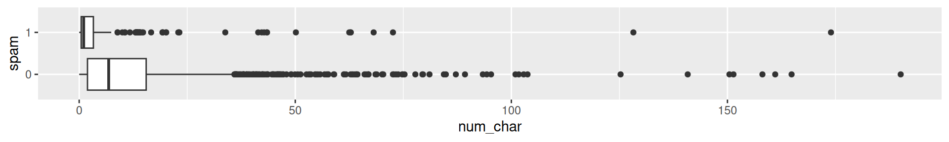
Would you expect spam to be longer or shorter?
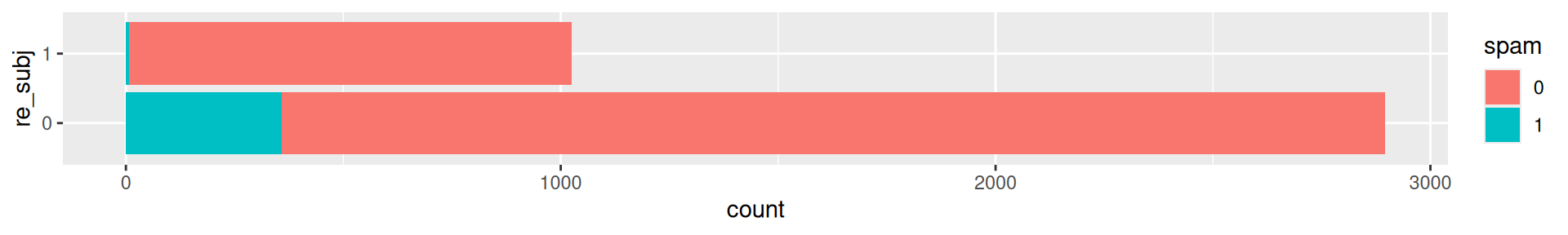
Would you expect spam subject to start with “Re:” or the like?
Both seem to give some signal. How can we model the relationship?
We focus first on just num_char:
email |> ggplot(aes(x = num_char, y = as.numeric(spam)-1)) +
geom_point(alpha = 0.2) + geom_smooth(method = "lm")
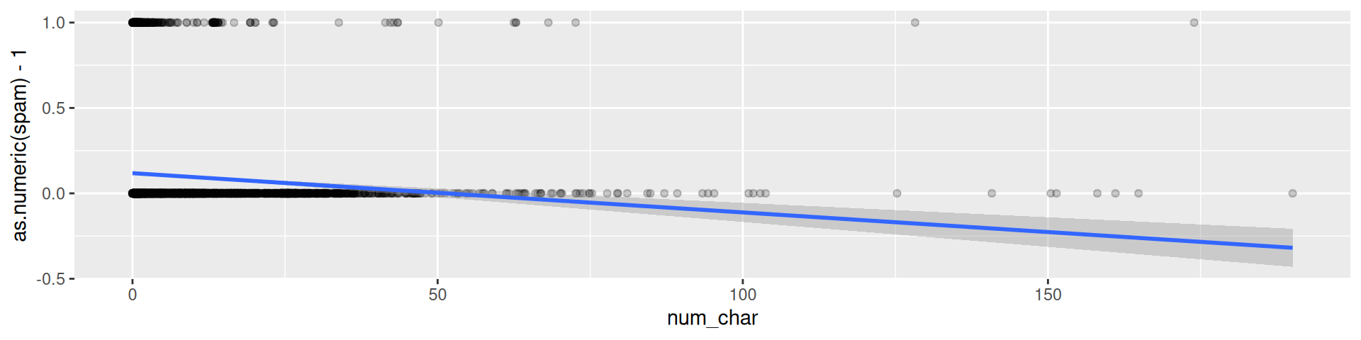
We would like to have a better concept!
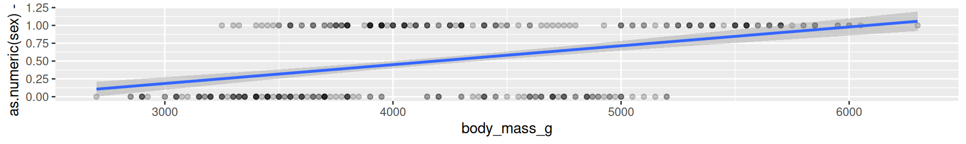
It does not make much sense to predict 0-1-values with a linear model.
\[ y_i ∼ \text{Bernoulli}(p_i) \]
All GLMs have the following three characteristics:
\[\text{logit}(p_i) = \log\left(\frac{p_i}{1-p_i}\right)\]
ggplot() +
geom_vline(xintercept = 0) + geom_hline(yintercept = 0) + geom_abline(intercept = 0, linetype = "dotted") +
geom_vline(xintercept = 1, linetype = "dashed") + geom_hline(yintercept = 1, linetype = "dashed") +
geom_function(fun = function(x) log(x/(1-x)), xlim=c(0.001,0.999), n = 500, color = "blue") +
geom_function(fun = function(x) 1/(1 + exp(-x)), color = "red") +
scale_x_continuous(breaks = seq(-4,4,1), limits = c(-4,4)) +
scale_y_continuous(breaks = seq(-4,4,1), limits = c(-4,4)) +
coord_fixed() + theme_minimal(base_size = 24) + labs(x = "x")
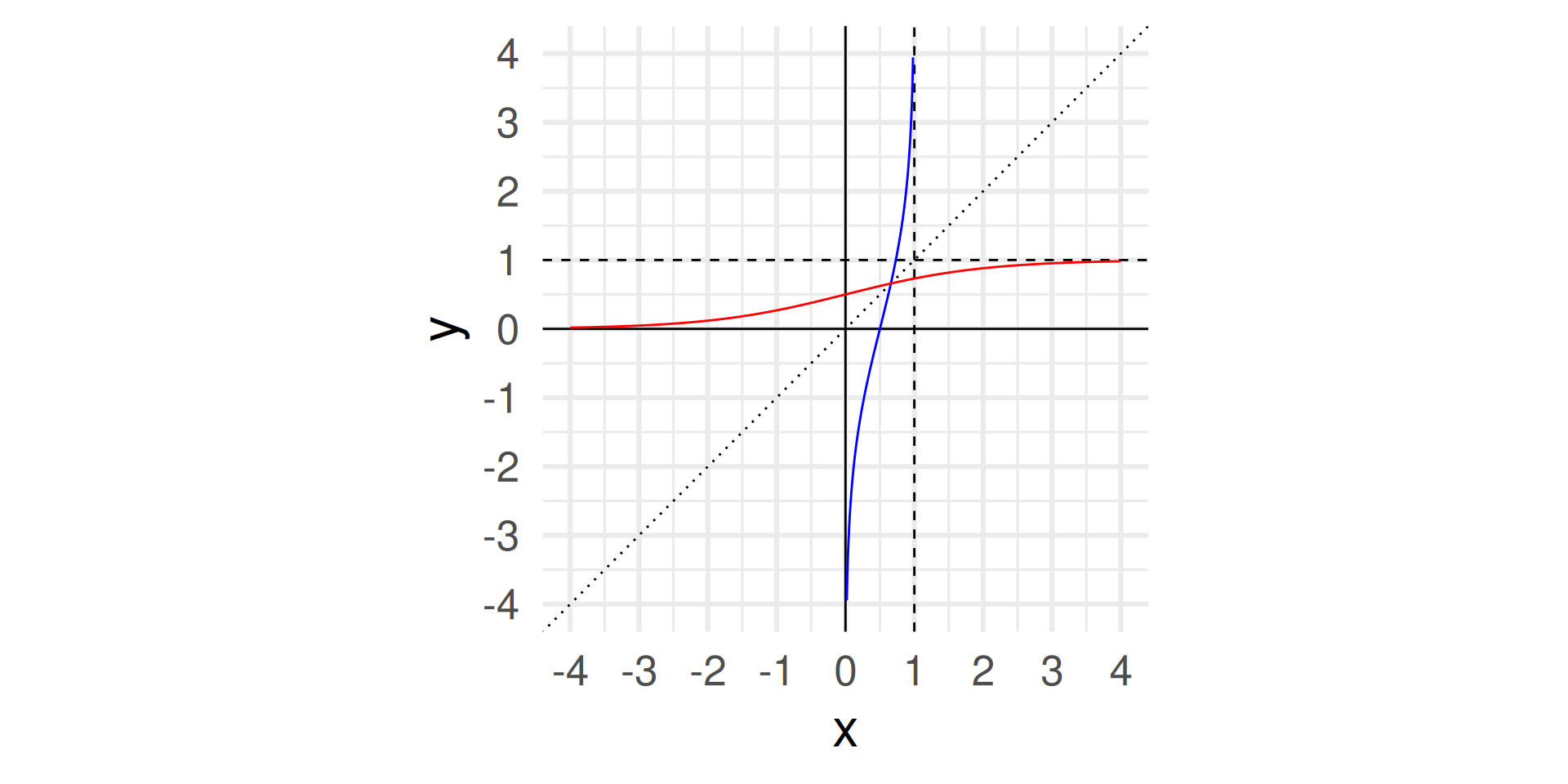
\[p_i = \frac{e^{\beta_0+\beta_1 x_{1,i} + \cdots + \beta_k x_{k,i}}}{1 + e^{\beta_0+\beta_1 x_{1,i} + \cdots + \beta_k x_{k,i}}}\]
With tidymodels we fit a GLM in the same way as a linear model except we
logistic_reg()"glm" instead of "lm" as the enginefamily = "binomial" for the link function to be used in the model# A tibble: 2 × 5
term estimate std.error statistic p.value
<chr> <dbl> <dbl> <dbl> <dbl>
1 (Intercept) -1.80 0.0716 -25.1 2.04e-139
2 num_char -0.0621 0.00801 -7.75 9.50e- 15
Model: \[\log\left(\frac{p}{1-p}\right) = -1.80-0.0621\cdot \text{num_char}\]
We can compute the predicted probability that an email with 2000 character is spam as follows: We plug in \(2\) for num_char (See slide before and note that num_char is in thousands.)
\[\log\left(\frac{p}{1-p}\right) = -1.80-0.0621\cdot 2 = -1.9242\]
Now, we solve for \(p\) by first exponentiation on both sides: \(\frac{p}{1-p} = e^{-1.9242} = 0.15\)
\[ \Rightarrow p = 0.15 \cdot (1 - p)\]
\[\Rightarrow p = 0.15 - 0.15\cdot p\] \[ \Rightarrow 1.15\cdot p = 0.15 \] \[\Rightarrow p = 0.15 / 1.15 = 0.13\]
logistic <- function(t) 1/(1+exp(-t))
preds <- tibble(x=c(2,15,40), y = logistic(-1.80-0.0621*x))
email |> ggplot(aes(x = num_char, y = as.numeric(spam)-1)) +
geom_point(alpha = 0.2) +
geom_function(fun = function(x) logistic(-1.80-0.0621*x),color="red") +
geom_point(data = preds, mapping = aes(x,y), color = "blue", size = 3)
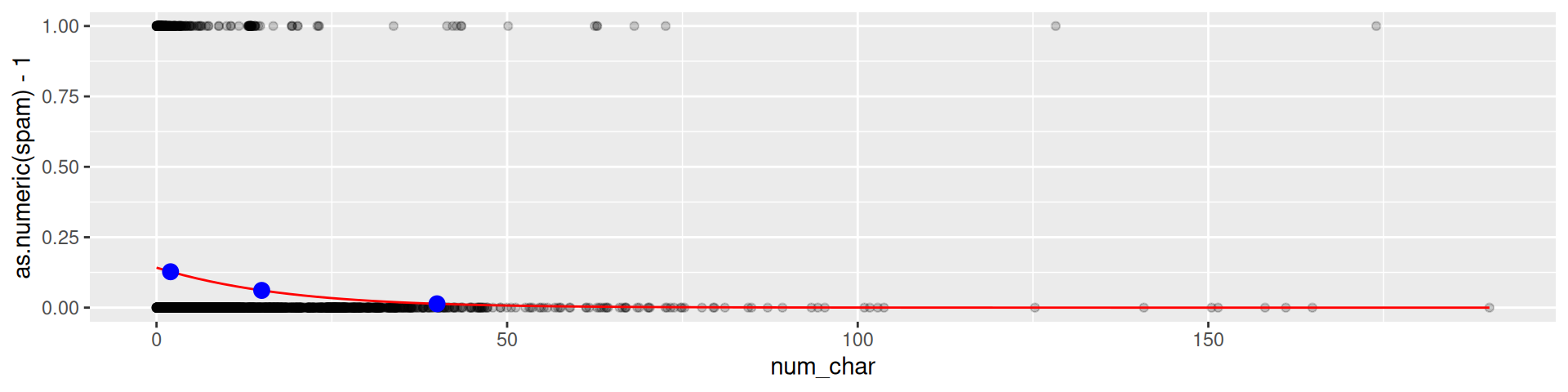
Spam probability 2,000 characters: 0.1273939
Spam probability 15,000 characters: 0.06114
Spam probability 40,000 characters: 0.0135999
\[\log\left(\frac{p}{1-p}\right) = -1.80-0.0621\cdot \text{num_char}\]
What does an increase by thousand characters (num_char + 1) imply?
Let us assume the predicted probability of an email is \(p_0\). Then an increase of num_char by one implied that the log-odds become
\[\log\left(\frac{p_0}{1-p_0}\right) - 0.0621 = \log\left(\frac{p_0}{1-p_0}\right) - \log(e^{0.0621})\]
\[ = \log\left(\frac{p_0}{1-p_0}\right) + \log(\frac{1}{e^{0.0621}}) = \log\left(\frac{p_0}{1-p_0} \frac{1}{e^{0.0621}}\right) = \log\left(\frac{p_0}{1-p_0} 0.94\right)\]
That means the odds of being spam decrease by 6%.
library(palmerpenguins)
sex_fit <- logistic_reg() |>
set_engine("glm") |>
fit(sex ~ body_mass_g, data = na.omit(penguins), family = "binomial")
tidy(sex_fit)# A tibble: 2 × 5
term estimate std.error statistic p.value
<chr> <dbl> <dbl> <dbl> <dbl>
1 (Intercept) -5.16 0.724 -7.13 1.03e-12
2 body_mass_g 0.00124 0.000173 7.18 7.10e-13
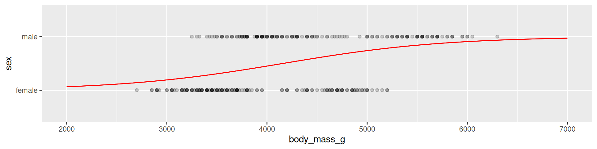
| Email labelled spam | Email labelled not spam | |
|---|---|---|
| Email is spam | True positive | False negative (Type 2 error) |
| Email is not spam | False positive (Type 1 error) | True negative |
More general: Confusion matrix of statistical classification:

Sensitivity is the true positive rate: TP / (TP + FN)
Specificity is the true negative rate: TN / (TN + FP)
For spam a positive case is an email labelled as spam:
Sensitivity: Fraction of emails labelled as spam among all emails which are spam.
Low sensitivity \(\to\) More false negatives \(\to\) More spam in you inbox!
Specificity: Fraction of emails labelled as not spam among all emails which are not spam.
Low specificity \(\to\) More false positives \(\to\) More relevant emails in spam folder!
If you were designing a spam filter, would you want sensitivity and specificity to be high or low? What are the trade-offs associated with each decision?
A COVID-19 test is called positive when it indicates the presence of the virus.
What is the sensitivity of a test?
Probability the test is positive when the person has COVID – True positive rate.
What is the specificity of a test?
Probability the test is negative when the person has no COVID – True negative rate.
Often the sensitivity is around 90% and the specificity is around 99%. What does that mean?
Explanation and Prediction are different Modelling Mindsets1.
Important: The mindsets are very different but they may use the same models!
logistic_reg() |>
set_engine("glm") |>
fit(spam ~ ., data = email, family = "binomial") |>
tidy() |> print(n = 22)Warning: glm.fit: fitted probabilities numerically 0 or 1 occurred
# A tibble: 22 × 5
term estimate std.error statistic p.value
<chr> <dbl> <dbl> <dbl> <dbl>
1 (Intercept) -9.09e+1 9.80e+3 -0.00928 9.93e- 1
2 to_multiple1 -2.68e+0 3.27e-1 -8.21 2.25e-16
3 from1 -2.19e+1 9.80e+3 -0.00224 9.98e- 1
4 cc 1.88e-2 2.20e-2 0.855 3.93e- 1
5 sent_email1 -2.07e+1 3.87e+2 -0.0536 9.57e- 1
6 time 8.48e-8 2.85e-8 2.98 2.92e- 3
7 image -1.78e+0 5.95e-1 -3.00 2.73e- 3
8 attach 7.35e-1 1.44e-1 5.09 3.61e- 7
9 dollar -6.85e-2 2.64e-2 -2.59 9.64e- 3
10 winneryes 2.07e+0 3.65e-1 5.67 1.41e- 8
11 inherit 3.15e-1 1.56e-1 2.02 4.32e- 2
12 viagra 2.84e+0 2.22e+3 0.00128 9.99e- 1
13 password -8.54e-1 2.97e-1 -2.88 4.03e- 3
14 num_char 5.06e-2 2.38e-2 2.13 3.35e- 2
15 line_breaks -5.49e-3 1.35e-3 -4.06 4.91e- 5
16 format1 -6.14e-1 1.49e-1 -4.14 3.53e- 5
17 re_subj1 -1.64e+0 3.86e-1 -4.25 2.16e- 5
18 exclaim_subj 1.42e-1 2.43e-1 0.585 5.58e- 1
19 urgent_subj1 3.88e+0 1.32e+0 2.95 3.18e- 3
20 exclaim_mess 1.08e-2 1.81e-3 5.98 2.23e- 9
21 numbersmall -1.19e+0 1.54e-1 -7.74 9.62e-15
22 numberbig -2.95e-1 2.20e-1 -1.34 1.79e- 1
In a one predictor model we can show both visually (This is simulated data)
lm_fit <- linear_reg() |>
set_engine("lm") |>
fit(y4 ~ x2, data = association)
loess_fit <- loess(y4 ~ x2, data = association)
loess_overfit <- loess(y4 ~ x2, span = 0.05, data = association)
association |>
select(x2, y4) |>
mutate(
Underfit = augment(lm_fit$fit) |> select(.fitted) |> pull(),
OK = augment(loess_fit) |> select(.fitted) |> pull(),
Overfit = augment(loess_overfit) |> select(.fitted) |> pull(),
) |>
pivot_longer(
cols = Underfit:Overfit,
names_to = "fit",
values_to = "y_hat"
) |>
mutate(fit = fct_relevel(fit, "Underfit", "OK", "Overfit")) |>
ggplot(aes(x = x2)) +
geom_point(aes(y = y4), color = "darkgray") +
geom_line(aes(y = y_hat, group = fit, color = fit), size = 1) +
labs(x = NULL, y = NULL, color = NULL) +
scale_color_viridis_d(option = "plasma", end = 0.7)
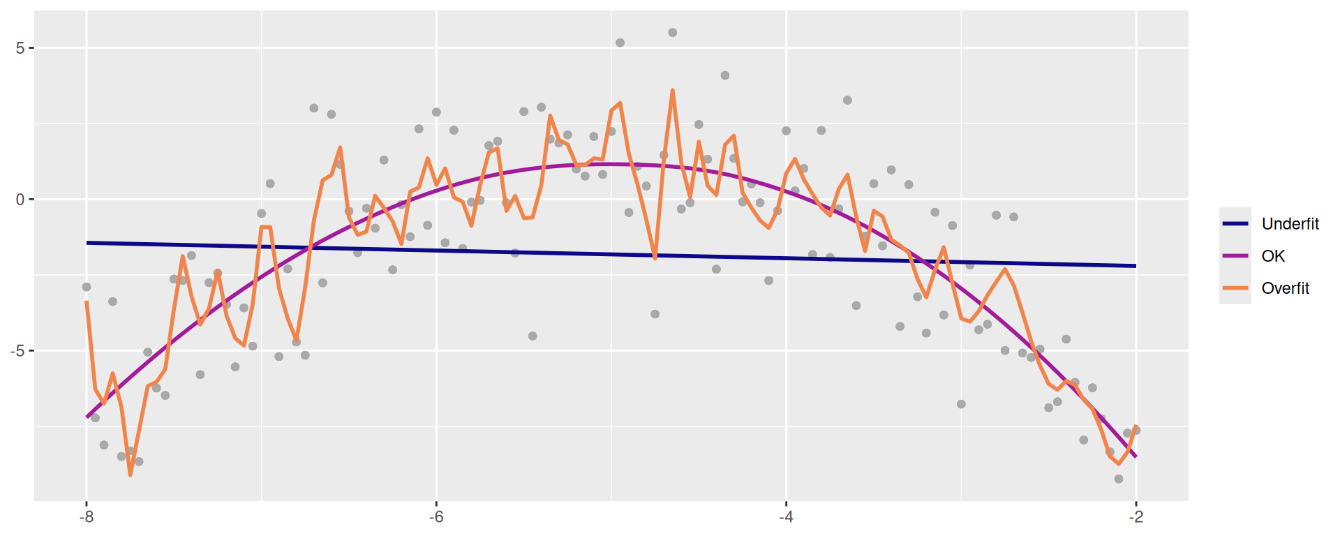
Problem:
Solution: We subsets our data for different tasks, as opposed to allocating all data to parameter estimation (as we have done so far).
Sidenote: Splitting data is very important for the predictive questions, because we want to know how well our model performs on new data. It is not relevant for explanatory questions where we want to interpret coefficients and infer about the underlying population.
# Fix random numbers by setting the seed
# Enables analysis to be reproducible when random numbers are used
set.seed(1116)
# Put 80% of the data into the training set
email_split <- initial_split(email, prop = 0.80)
# Create data frames for the two sets:
train_data <- training(email_split)
test_data <- testing(email_split)A note on the seed: The seed is an arbitrary number that is used to initialize a pseudorandom number generator. The same seed will always result in the same sequence of pseudorandom numbers. This is useful for reproducibility.
Rows: 3,136
Columns: 21
$ spam <fct> 0, 1, 0, 1, 0, 0, 0, 0, 0, 0, 1, 0, 0, 0, 0, 0, 0, 0, 0, …
$ to_multiple <fct> 0, 0, 0, 0, 1, 1, 0, 0, 0, 0, 0, 0, 0, 1, 0, 0, 0, 0, 0, …
$ from <fct> 1, 1, 1, 1, 1, 1, 1, 1, 1, 1, 1, 1, 1, 1, 1, 1, 1, 1, 1, …
$ cc <int> 2, 0, 0, 0, 0, 0, 0, 0, 0, 0, 0, 0, 0, 35, 0, 0, 0, 0, 0,…
$ sent_email <fct> 1, 0, 1, 0, 0, 0, 0, 0, 0, 0, 0, 0, 0, 0, 1, 0, 0, 0, 0, …
$ time <dttm> 2012-01-25 23:46:55, 2012-01-03 06:28:28, 2012-02-04 17:…
$ image <dbl> 0, 0, 0, 0, 0, 1, 0, 0, 0, 0, 0, 0, 0, 0, 0, 0, 0, 0, 0, …
$ attach <dbl> 0, 0, 0, 0, 0, 1, 0, 0, 0, 0, 0, 0, 0, 0, 0, 0, 0, 0, 0, …
$ dollar <dbl> 10, 0, 0, 0, 0, 0, 13, 0, 0, 0, 2, 0, 0, 0, 14, 0, 0, 0, …
$ winner <fct> no, no, no, no, no, no, no, yes, no, no, no, no, no, no, …
$ inherit <dbl> 0, 0, 0, 0, 0, 1, 0, 0, 0, 0, 0, 0, 0, 0, 0, 0, 0, 0, 0, …
$ viagra <dbl> 0, 0, 0, 0, 0, 0, 0, 0, 0, 0, 0, 0, 0, 0, 0, 0, 0, 0, 0, …
$ password <dbl> 0, 0, 0, 0, 0, 0, 0, 0, 0, 0, 0, 0, 0, 0, 0, 0, 3, 0, 0, …
$ num_char <dbl> 23.308, 1.162, 4.732, 42.238, 1.228, 25.599, 16.764, 10.7…
$ line_breaks <int> 477, 2, 127, 712, 30, 674, 367, 226, 98, 671, 46, 192, 67…
$ format <fct> 1, 0, 1, 1, 0, 1, 1, 1, 1, 1, 0, 1, 0, 0, 1, 1, 1, 1, 1, …
$ re_subj <fct> 1, 0, 1, 0, 0, 0, 0, 0, 0, 0, 0, 0, 1, 0, 1, 0, 0, 0, 1, …
$ exclaim_subj <dbl> 0, 0, 0, 0, 0, 0, 1, 0, 0, 0, 1, 0, 0, 0, 0, 0, 0, 0, 1, …
$ urgent_subj <fct> 0, 0, 0, 0, 0, 0, 0, 0, 0, 0, 0, 0, 0, 0, 0, 0, 0, 0, 0, …
$ exclaim_mess <dbl> 12, 0, 2, 2, 2, 31, 2, 0, 0, 1, 0, 1, 2, 0, 2, 0, 11, 1, …
$ number <fct> small, none, big, big, small, small, small, small, small,…
Rows: 785
Columns: 21
$ spam <fct> 0, 0, 0, 0, 0, 0, 0, 0, 0, 0, 0, 0, 0, 0, 0, 0, 0, 0, 0, …
$ to_multiple <fct> 1, 0, 0, 0, 0, 0, 0, 0, 0, 0, 1, 0, 0, 1, 0, 0, 0, 0, 0, …
$ from <fct> 1, 1, 1, 1, 1, 1, 1, 1, 1, 1, 1, 1, 1, 1, 1, 1, 1, 1, 1, …
$ cc <int> 0, 1, 0, 1, 4, 0, 0, 0, 0, 0, 0, 0, 0, 0, 0, 0, 0, 3, 0, …
$ sent_email <fct> 1, 1, 0, 0, 0, 0, 0, 0, 0, 0, 0, 0, 0, 0, 0, 0, 0, 1, 0, …
$ time <dttm> 2012-01-01 18:55:06, 2012-01-01 20:38:32, 2012-01-02 06:…
$ image <dbl> 0, 0, 0, 0, 0, 0, 0, 0, 0, 0, 0, 0, 0, 0, 0, 0, 1, 0, 0, …
$ attach <dbl> 0, 0, 0, 0, 0, 0, 0, 0, 0, 0, 0, 0, 0, 1, 0, 0, 1, 0, 0, …
$ dollar <dbl> 0, 0, 5, 0, 0, 0, 0, 5, 4, 0, 0, 0, 21, 0, 0, 2, 9, 0, 0,…
$ winner <fct> no, no, no, no, no, no, no, no, no, no, no, no, no, no, n…
$ inherit <dbl> 0, 0, 0, 0, 0, 0, 0, 0, 1, 0, 0, 0, 0, 0, 0, 0, 0, 0, 0, …
$ viagra <dbl> 0, 0, 0, 0, 0, 0, 0, 0, 0, 0, 0, 0, 0, 0, 0, 0, 0, 0, 0, …
$ password <dbl> 0, 0, 1, 0, 0, 0, 0, 0, 0, 1, 0, 0, 0, 0, 0, 0, 0, 0, 2, …
$ num_char <dbl> 4.837, 15.075, 18.037, 45.842, 11.438, 1.482, 14.431, 0.9…
$ line_breaks <int> 193, 354, 345, 881, 125, 24, 296, 13, 192, 14, 32, 30, 55…
$ format <fct> 1, 1, 1, 1, 0, 1, 1, 0, 1, 0, 0, 0, 1, 1, 1, 1, 1, 1, 1, …
$ re_subj <fct> 0, 1, 0, 1, 1, 0, 0, 0, 0, 0, 1, 0, 0, 0, 1, 0, 0, 1, 0, …
$ exclaim_subj <dbl> 0, 0, 1, 0, 0, 0, 0, 0, 0, 0, 0, 0, 0, 0, 0, 0, 0, 0, 0, …
$ urgent_subj <fct> 0, 0, 0, 0, 0, 0, 0, 0, 0, 0, 0, 0, 0, 0, 0, 0, 0, 0, 0, …
$ exclaim_mess <dbl> 1, 10, 20, 5, 2, 0, 0, 0, 6, 0, 0, 1, 3, 0, 4, 0, 1, 0, 1…
$ number <fct> big, small, small, big, small, none, small, small, small,…
email_fit <- logistic_reg() |>
set_engine("glm") |>
fit(spam ~ ., data = train_data, family = "binomial")Warning: glm.fit: fitted probabilities numerically 0 or 1 occurred
We get a warning and should explore the reasons for 0 or 1 probability.
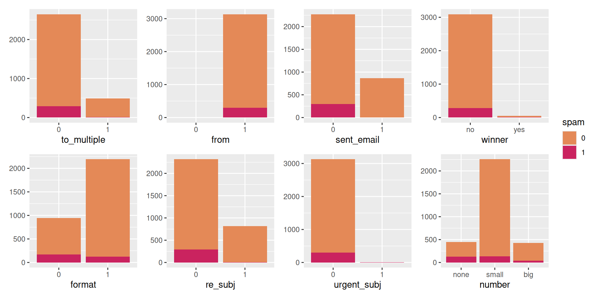
Closer look at from and sent_email.
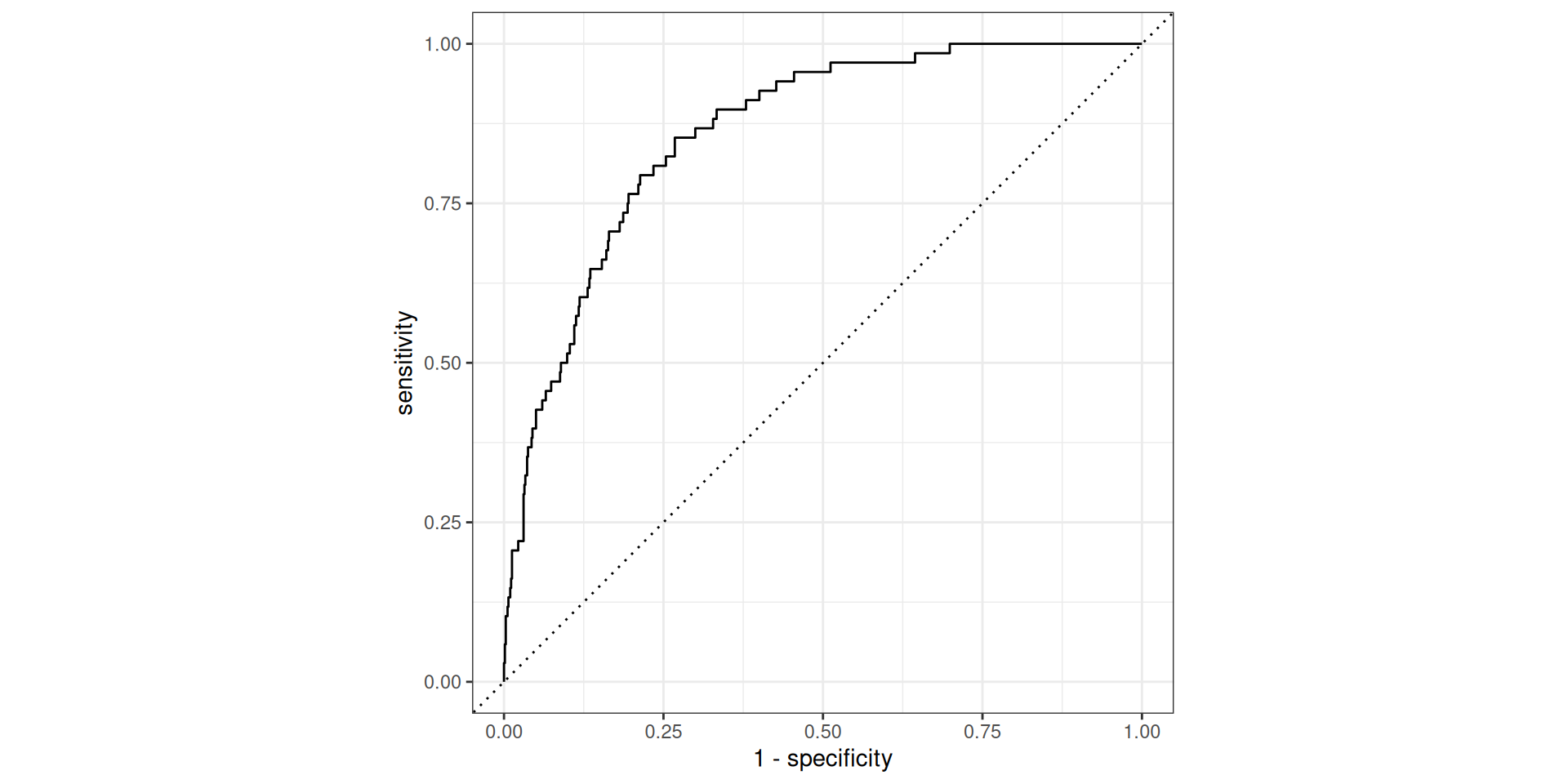
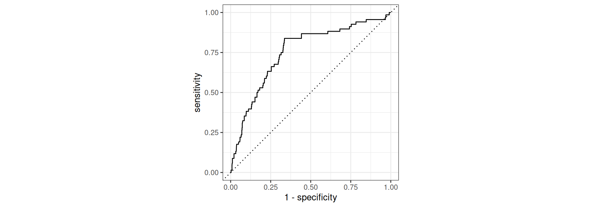
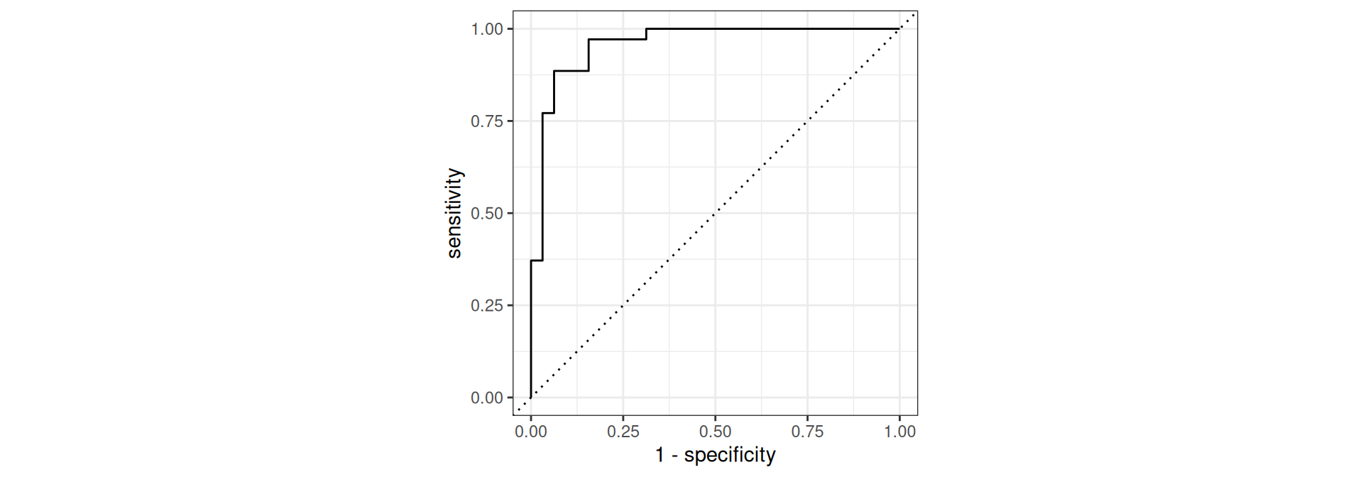
from: Whether the message was listed as from anyone (this is usually set by default for regular outgoing email).
# A tibble: 3 × 3
spam from n
<fct> <fct> <int>
1 0 1 2837
2 1 0 3
3 1 1 296
No non-spam mails without from.
# A tibble: 22 × 4
# Groups: name [11]
name spam mean sd
<chr> <fct> <dbl> <dbl>
1 attach 0 0.124 0.775
2 attach 1 0.227 0.620
3 cc 0 0.393 2.62
4 cc 1 0.388 3.25
5 dollar 0 1.56 5.33
6 dollar 1 0.779 3.01
7 exclaim_mess 0 6.68 50.2
8 exclaim_mess 1 8.75 88.4
9 exclaim_subj 0 0.0783 0.269
10 exclaim_subj 1 0.0769 0.267
11 image 0 0.0536 0.503
12 image 1 0.00334 0.0578
13 inherit 0 0.0352 0.216
14 inherit 1 0.0702 0.554
15 line_breaks 0 247. 326.
16 line_breaks 1 108. 321.
17 num_char 0 11.4 14.9
18 num_char 1 5.63 15.7
19 password 0 0.112 0.938
20 password 1 0.0201 0.182
21 viagra 0 0 0
22 viagra 1 0.0268 0.463
viagra has no mentions in non-spam emails.
email_fit <- logistic_reg() |>
set_engine("glm") |>
fit(spam ~ . - from - sent_email - viagra, data = train_data, family = "binomial") Warning: glm.fit: fitted probabilities numerically 0 or 1 occurred
parsnip model object
Call: stats::glm(formula = spam ~ . - from - sent_email - viagra, family = stats::binomial,
data = data)
Coefficients:
(Intercept) to_multiple1 cc time image
-9.867e+01 -2.505e+00 1.944e-02 7.396e-08 -2.854e+00
attach dollar winneryes inherit password
5.070e-01 -6.440e-02 2.170e+00 4.499e-01 -7.065e-01
num_char line_breaks format1 re_subj1 exclaim_subj
5.870e-02 -5.420e-03 -9.017e-01 -2.995e+00 1.002e-01
urgent_subj1 exclaim_mess numbersmall numberbig
3.572e+00 1.009e-02 -8.518e-01 -1.329e-01
Degrees of Freedom: 3135 Total (i.e. Null); 3117 Residual
Null Deviance: 1974
Residual Deviance: 1447 AIC: 1485
We still get a warning, but without very high coefficients.
Predicting the raw values (log-odds)
1 2 3 4 5 6
-4.942500 -6.312226 -3.938487 -6.688992 -4.399541 -1.587700
Predicting probabilities
email_pred <-
predict(email_fit, test_data, type = "prob") |>
select(spam_prob = .pred_1) |>
mutate(spam_logodds =
predict(email_fit, test_data, type = "raw"),
spam_odds = exp(spam_logodds)) |>
bind_cols(predict(email_fit, test_data)) |>
# Append real data
bind_cols(test_data |> select(spam))
email_pred# A tibble: 785 × 5
spam_prob spam_logodds spam_odds .pred_class spam
<dbl> <dbl> <dbl> <fct> <fct>
1 0.00709 -4.94 0.00714 0 0
2 0.00181 -6.31 0.00181 0 0
3 0.0191 -3.94 0.0195 0 0
4 0.00124 -6.69 0.00124 0 0
5 0.0121 -4.40 0.0123 0 0
6 0.170 -1.59 0.204 0 0
7 0.0410 -3.15 0.0427 0 0
8 0.139 -1.83 0.161 0 0
9 0.0617 -2.72 0.0657 0 0
10 0.0983 -2.22 0.109 0 0
# ℹ 775 more rows
predict..pred_class prediction is when the probability > 0.5.
Answers: odds > 1, log-odds > 0
# A tibble: 785 × 5
spam_prob spam_logodds spam_odds .pred_class spam
<dbl> <dbl> <dbl> <fct> <fct>
1 0.903 2.23 9.29 1 1
2 0.833 1.60 4.98 1 0
3 0.825 1.55 4.71 1 1
4 0.733 1.01 2.75 1 1
5 0.683 0.766 2.15 1 1
6 0.626 0.517 1.68 1 1
7 0.614 0.464 1.59 1 0
8 0.597 0.392 1.48 1 1
9 0.538 0.153 1.17 1 1
10 0.537 0.148 1.16 1 0
11 0.510 0.0404 1.04 1 0
12 0.491 -0.0345 0.966 0 0
13 0.490 -0.0407 0.960 0 0
14 0.489 -0.0453 0.956 0 1
15 0.483 -0.0698 0.933 0 1
16 0.473 -0.107 0.899 0 0
17 0.463 -0.150 0.861 0 0
18 0.457 -0.174 0.840 0 0
19 0.447 -0.212 0.809 0 0
20 0.447 -0.214 0.808 0 1
# ℹ 765 more rows
We see false positives and false negatives.
Receiver operating characteristic (ROC) curve1 which plots true positive rate (sensitivity) vs. false positive rate (1 - specificity)
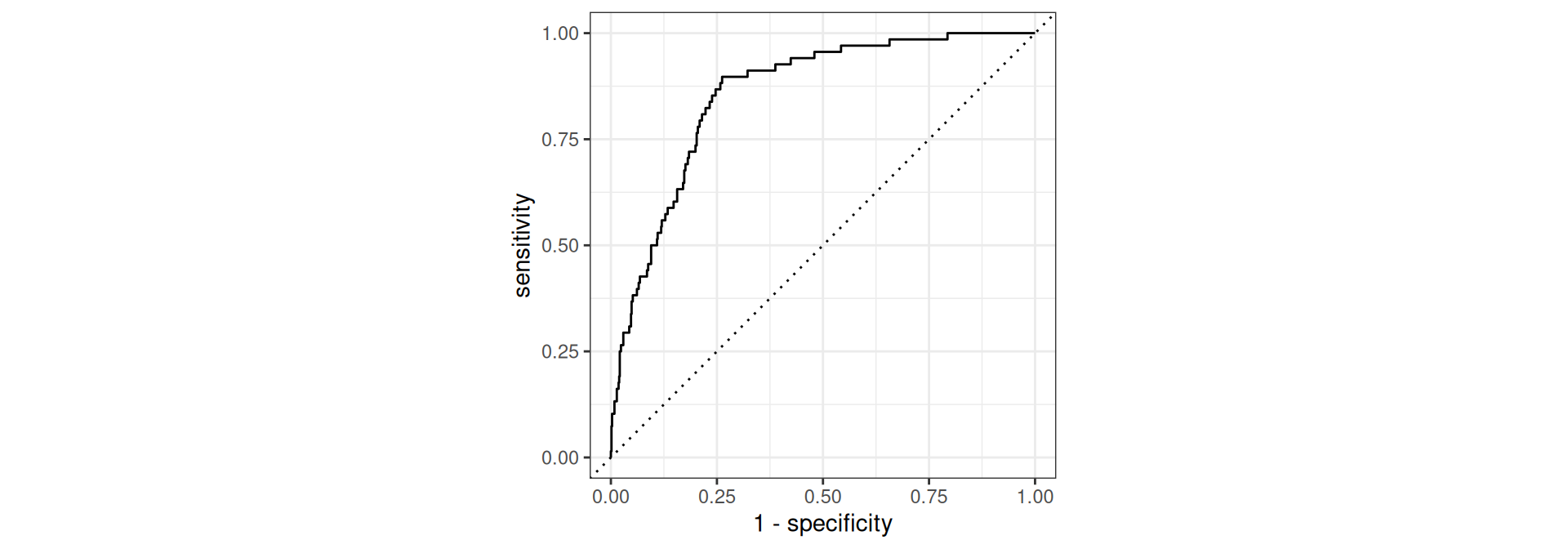
email_pred_roc <- email_pred |> roc_curve(
truth = spam, spam_prob,
event_level = "second" # this adjusts the location above the diagonal
)
email_pred_roc_thresholds <- email_pred_roc |>
mutate(.threshold_rounded = round(.threshold, digits = 2)) |>
filter(.threshold_rounded == 0.25 | .threshold_rounded == 0.5 | .threshold_rounded == 0.75)
email_pred_roc |>
ggplot(aes(x = 1 - specificity, y = sensitivity)) + geom_line() +
geom_point(data = email_pred_roc |> slice(round(seq(30,nrow(email_pred_roc)-30, length.out = 10))),
color = "black") +
geom_text(data = email_pred_roc |> slice(round(seq(30,nrow(email_pred_roc)-30, length.out = 10))),
mapping = aes(label = round(.threshold, digits = 2)),
color = "black",
nudge_x = 0.04,
nudge_y = -0.03, size = 3) +
geom_abline(lty = 3) +
labs(title = "ROC-curve") +
coord_equal() +
theme_bw()Find the area under the curve (AUC).
In calculus language:
\(\int_0^1 \text{TPR}(\text{FPR}) d\text{FPR}\)
Remember:
Create a recipe for feature engineering steps to be applied to the training data
tidymodels way (similar to a pipeline in python’s scikit-learn).Fit the model to the training data after these steps have been applied
Using the model estimates from the training data, predict outcomes for the test data
Evaluate the performance of the model on the test data
email_rec <- recipe(
spam ~ ., # formula
data = train_data # data to use for cataloguing names and types of variables
)
summary(email_rec) |> print(n = 21)# A tibble: 21 × 4
variable type role source
<chr> <list> <chr> <chr>
1 to_multiple <chr [3]> predictor original
2 from <chr [3]> predictor original
3 cc <chr [2]> predictor original
4 sent_email <chr [3]> predictor original
5 time <chr [1]> predictor original
6 image <chr [2]> predictor original
7 attach <chr [2]> predictor original
8 dollar <chr [2]> predictor original
9 winner <chr [3]> predictor original
10 inherit <chr [2]> predictor original
11 viagra <chr [2]> predictor original
12 password <chr [2]> predictor original
13 num_char <chr [2]> predictor original
14 line_breaks <chr [2]> predictor original
15 format <chr [3]> predictor original
16 re_subj <chr [3]> predictor original
17 exclaim_subj <chr [2]> predictor original
18 urgent_subj <chr [3]> predictor original
19 exclaim_mess <chr [2]> predictor original
20 number <chr [3]> predictor original
21 spam <chr [3]> outcome original
The object email_rec only includes meta-data (columns names and types)!
step_date can easily extract theseall_nominal or all_outcomes from tidymodels for column selection.Variables that contain only a single value.
email_rec <- recipe(
spam ~ ., # formula
data = train_data # data to use for cataloguing names and types of variables
) |>
step_rm(from, sent_email, viagra) |>
step_date(time, features = c("dow", "month")) |>
step_rm(time) |>
step_dummy(all_nominal(), -all_outcomes()) |>
step_zv(all_predictors())
print(email_rec)
── Recipe ──────────────────────────────────────────────────────────────────────
── Inputs
Number of variables by role
outcome: 1
predictor: 20
── Operations
• Variables removed: from, sent_email, viagra
• Date features from: time
• Variables removed: time
• Dummy variables from: all_nominal() and -all_outcomes()
• Zero variance filter on: all_predictors()
The object email_rec only includes meta-data of the data frame it shall work on (a formula, columns names and types)!
Workflows bring together models and recipes so that they can be easily applied to both the training and test data.
══ Workflow ════════════════════════════════════════════════════════════════════
Preprocessor: Recipe
Model: logistic_reg()
── Preprocessor ────────────────────────────────────────────────────────────────
5 Recipe Steps
• step_rm()
• step_date()
• step_rm()
• step_dummy()
• step_zv()
── Model ───────────────────────────────────────────────────────────────────────
Logistic Regression Model Specification (classification)
Computational engine: glm
# A tibble: 27 × 5
term estimate std.error statistic p.value
<chr> <dbl> <dbl> <dbl> <dbl>
1 (Intercept) -0.651 0.254 -2.57 1.03e- 2
2 cc 0.0214 0.0229 0.936 3.49e- 1
3 image -2.99 1.31 -2.28 2.28e- 2
4 attach 0.512 0.116 4.41 1.03e- 5
5 dollar -0.0651 0.0307 -2.12 3.40e- 2
6 inherit 0.440 0.205 2.15 3.14e- 2
7 password -0.723 0.302 -2.39 1.67e- 2
8 num_char 0.0585 0.0240 2.43 1.50e- 2
9 line_breaks -0.00548 0.00139 -3.94 8.24e- 5
10 exclaim_subj 0.0998 0.268 0.373 7.09e- 1
11 exclaim_mess 0.0103 0.00198 5.20 2.02e- 7
12 to_multiple_X1 -2.56 0.339 -7.56 4.11e-14
13 winner_yes 2.24 0.430 5.21 1.90e- 7
14 format_X1 -0.953 0.157 -6.06 1.38e- 9
15 re_subj_X1 -3.00 0.444 -6.76 1.39e-11
16 urgent_subj_X1 3.69 1.15 3.20 1.37e- 3
17 number_small -0.840 0.162 -5.20 1.98e- 7
18 number_big -0.0915 0.244 -0.375 7.07e- 1
19 time_dow_Mon -0.326 0.303 -1.08 2.82e- 1
20 time_dow_Tue 0.0813 0.275 0.296 7.67e- 1
21 time_dow_Wed -0.260 0.275 -0.946 3.44e- 1
22 time_dow_Thu -0.220 0.279 -0.788 4.31e- 1
23 time_dow_Fri -0.0612 0.275 -0.223 8.24e- 1
24 time_dow_Sat 0.0646 0.292 0.221 8.25e- 1
25 time_month_Feb 0.760 0.178 4.26 2.03e- 5
26 time_month_Mar 0.506 0.178 2.85 4.40e- 3
27 time_month_Apr -12.0 394. -0.0306 9.76e- 1
# A tibble: 785 × 23
.pred_0 .pred_1 spam to_multiple from cc sent_email time
<dbl> <dbl> <fct> <fct> <fct> <int> <fct> <dttm>
1 0.993 0.00653 0 1 1 0 1 2012-01-01 18:55:06
2 0.998 0.00169 0 0 1 1 1 2012-01-01 20:38:32
3 0.987 0.0127 0 0 1 0 0 2012-01-02 06:42:16
4 0.999 0.000825 0 0 1 1 0 2012-01-02 16:12:51
5 0.991 0.00876 0 0 1 4 0 2012-01-02 17:45:36
6 0.878 0.122 0 0 1 0 0 2012-01-02 22:55:03
7 0.959 0.0414 0 0 1 0 0 2012-01-03 02:07:17
8 0.852 0.148 0 0 1 0 0 2012-01-03 06:41:35
9 0.938 0.0619 0 0 1 0 0 2012-01-03 17:02:35
10 0.896 0.104 0 0 1 0 0 2012-01-03 12:14:51
# ℹ 775 more rows
# ℹ 15 more variables: image <dbl>, attach <dbl>, dollar <dbl>, winner <fct>,
# inherit <dbl>, viagra <dbl>, password <dbl>, num_char <dbl>,
# line_breaks <int>, format <fct>, re_subj <fct>, exclaim_subj <dbl>,
# urgent_subj <fct>, exclaim_mess <dbl>, number <fct>
# A tibble: 1 × 3
.metric .estimator .estimate
<chr> <chr> <dbl>
1 roc_auc binary 0.860
This is better than our former model (without the feature engineering workflow), which had AUC = 0.857.
Suppose we decide to label an email as spam if the model predicts the probability of spam to be more than 0.5. (That is the default.)
Confusion matrix:
cutoff_prob <- 0.5
email_pred |>
mutate(
spam = if_else(spam == 1, "Email is spam", "Email is not spam"),
spam_pred = if_else(.pred_1 > cutoff_prob, "Email labelled spam", "Email labelled not spam")
) |>
count(spam_pred, spam) |>
pivot_wider(names_from = spam_pred, values_from = n) |>
select(1,3,2) |> slice(c(2,1)) |> # reorder rows and cols to fit convention
knitr::kable()| spam | Email labelled spam | Email labelled not spam |
|---|---|---|
| Email is spam | 14 | 54 |
| Email is not spam | 10 | 707 |
Sensitivity: 14/(14+54) = 0.206
Specificity: 707/(707+10) = 0.986
Suppose we decide to label an email as spam if the model predicts the probability of spam to be more than 0.25.
Confusion matrix:
| spam | Email labelled spam | Email labelled not spam |
|---|---|---|
| Email is spam | 32 | 36 |
| Email is not spam | 61 | 656 |
Sensitivity: 32/(32+36) = 0.471
Specificity: 656/(656 + 61) = 0.915
Suppose we decide to label an email as spam if the model predicts the probability of spam to be more than 0.75.
Confusion matrix:
| spam | Email labelled spam | Email labelled not spam |
|---|---|---|
| Email is spam | 3 | 65 |
| Email is not spam | 1 | 716 |
Sensitivity: 3/(3+65) = 0.044
Specificity: 716/(716+1) = 0.999
We make a new simple recipe and draw workflow and fitting re-using the same specified logisitc regression model email_mod.
simple_email_rec <- recipe(
spam ~ num_char, # formula
data = train_data # data to use for cataloguing names and types of variables
)
simple_email_pred <-
workflow() |>
add_model(email_mod) |>
add_recipe(simple_email_rec) |>
fit(data = train_data) |>
predict(test_data, type = "prob") |>
bind_cols(test_data |> select(spam,num_char,time))
simple_email_pred # A tibble: 785 × 5
.pred_0 .pred_1 spam num_char time
<dbl> <dbl> <fct> <dbl> <dttm>
1 0.889 0.111 0 4.84 2012-01-01 18:55:06
2 0.936 0.0644 0 15.1 2012-01-01 20:38:32
3 0.945 0.0547 0 18.0 2012-01-02 06:42:16
4 0.989 0.0113 0 45.8 2012-01-02 16:12:51
5 0.922 0.0784 0 11.4 2012-01-02 17:45:36
6 0.868 0.132 0 1.48 2012-01-02 22:55:03
7 0.933 0.0667 0 14.4 2012-01-03 02:07:17
8 0.864 0.136 0 0.978 2012-01-03 06:41:35
9 0.905 0.0953 0 7.79 2012-01-03 17:02:35
10 0.864 0.136 0 0.978 2012-01-03 12:14:51
# ℹ 775 more rows
# A tibble: 1 × 3
.metric .estimator .estimate
<chr> <chr> <dbl>
1 roc_auc binary 0.753
Conclusion: It is not as good compared to AUC 0.86
Following all the steps introduced before:
set.seed(1)
# Put 80% of the data into the training set
peng_split <- initial_split(penguins, prop = 0.80)
# Create data frames for the two sets:
train_data_peng <- training(peng_split)
test_data_peng <- testing(peng_split)
# Create a recipe for the model
peng_rec <- recipe(
sex ~ .,
data = train_data_peng
) |>
step_naomit(all_predictors()) |>
step_dummy(all_nominal(), -all_outcomes()) |>
step_zv(all_predictors())
# Create a logistic regression model
peng_mod <- logistic_reg() |>
set_engine("glm")
# Create a workflow
peng_wflow <- workflow() |>
add_model(peng_mod) |>
add_recipe(peng_rec)
# Fitting model to training data
peng_fit <- peng_wflow |>
fit(data = train_data_peng)
# Make predictions for test data
peng_pred <- peng_fit |>
predict(test_data_peng, type = "prob") |>
bind_cols(test_data_peng)Confusion matrix:
cutoff_prob <- 0.5
peng_pred |>
mutate(
sex = if_else(sex == "male", "Penguin is male", "Penguin is female"),
sex_pred = if_else(.pred_male > cutoff_prob, "Penguin labelled male", "Penguin labelled female")
) |>
count(sex_pred, sex) |>
pivot_wider(names_from = sex_pred, values_from = n) |>
select(1,3,2) |> slice(c(2,1)) |> # reorder rows and cols to fit convention
knitr::kable()| sex | Penguin labelled male | Penguin labelled female |
|---|---|---|
| Penguin is male | 31 | 4 |
| Penguin is female | 4 | 28 |
Sensitivity: 31/(31+4) = 0.886
Specificity: 28/(28+4) = 0.875
Confusion matrix:
cutoff_prob <- 0.25
peng_pred |>
mutate(
sex = if_else(sex == "male", "Penguin is male", "Penguin is female"),
sex_pred = if_else(.pred_male > cutoff_prob, "Penguin labelled male", "Penguin labelled female")
) |>
count(sex_pred, sex) |>
pivot_wider(names_from = sex_pred, values_from = n) |>
select(1,3,2) |> slice(c(2,1)) |> # reorder rows and cols to fit convention
knitr::kable()| sex | Penguin labelled male | Penguin labelled female |
|---|---|---|
| Penguin is male | 34 | 1 |
| Penguin is female | 7 | 25 |
Sensitivity: 34/(34+1) = 0.971
Specificity: 25/(25+7) = 0.781
Confusion matrix:
cutoff_prob <- 0.75
peng_pred |>
mutate(
sex = if_else(sex == "male", "Penguin is male", "Penguin is female"),
sex_pred = if_else(.pred_male > cutoff_prob, "Penguin labelled male", "Penguin labelled female")
) |>
count(sex_pred, sex) |>
pivot_wider(names_from = sex_pred, values_from = n) |>
select(1,3,2) |> slice(c(2,1)) |> # reorder rows and cols to fit convention
knitr::kable()| sex | Penguin labelled male | Penguin labelled female |
|---|---|---|
| Penguin is male | 29 | 6 |
| Penguin is female | 2 | 30 |
Sensitivity: 29/(29+6) = 0.829
Specificity: 30/(30+2) = 0.938

MDSSB-DSCO-02: Data Science Concepts