W#09: Hypothesis Testing, Classification and Regression with Decision Trees, Overfitting

Jan Lorenz

Table of contents

• Hypothesis testing
• Simulation for Hypothesis Testing
• p-value
• Classification: Compare logistic regression and decision tree
• Regression: Compare linear regression and decision tree
• Overfitting with decision trees
• What do we mean by “model”? How to be specific

Packages used here

library(tidyverse)
library(tidymodels)
library(rpart.plot)
library(openintro)
library(palmerpenguins)

Hypothesis testing

Large part of the content adapted from http://datasciencebox.org.

Organ donors

Background story: People providing an organ for donation sometimes seek the help of a special “medical consultant”. These consultants assist the patient in all aspects of the surgery, with the goal of reducing the possibility of complications during the medical procedure and recovery. Patients might choose a consultant based in part on the historical complication rate of the consultant’s clients.

Example track record: One consultant tried to attract patients by noting that the average complication rate for liver donor surgeries in the US is about 10%, but her clients have only had 3 complications in the 62 liver donor surgeries she has facilitated. She claims this is strong evidence that her work meaningfully contributes to reducing complications (and therefore she should be hired!).

Is this strong evidence for a good track record?

Data

organ_donor <- tibble(
  outcome = c(rep("complication", 3), rep("no complication", 59))
)

organ_donor |>
  count(outcome)

# A tibble: 2 × 2
  outcome             n
  <chr>           <int>
1 complication        3
2 no complication    59

Parameter vs. statistic

A parameter for a hypothesis test is the “true” value of interest. We typically estimate the parameter using a sample statistic as a point estimate.

\(q\): true rate of complication, here 0.1 (10% complication rate in US)

\(\hat{q}\): rate of complication in the sample = \(\frac{3}{62}\) = 0.048 (This is the point estimate.)

Correlation vs. causation

Is it possible to infer the consultant’s claim using the data?

No. The claim is: There is a causal connection. However, the data are observational. For example, maybe patients who can afford a medical consultant can afford better medical care, which can also lead to a lower complication rate (for example).

What is possible?

While it is not possible to assess the causal claim, it is still possible to test for an association using these data. For this question we ask, could the low complication rate of \(\hat{q}\) = 0.048 be due to chance?

Two claims

• Null hypothesis \(H_0\): “There is nothing going on”

Complication rate for this consultant is no different than the US average of 10%

• Alternative hypothesis \(H_1\): “There is something going on”

Complication rate for this consultant is lower than the US average of 10%

Understand hypothesis testing as a court trial

• Null hypothesis, \(H_0\): Defendant is innocent

• Alternative hypothesis, \(H_A\): Defendant is guilty

• Present the evidence: Collect data

• Judge the evidence: “Could these data plausibly have happened by chance if the null hypothesis were true?”

  • Yes: Fail to reject \(H_0\)
  • No: Reject \(H_0\)

Hypothesis testing framework

• Start with a null hypothesis, \(H_0\), that represents the status quo

• Set an alternative hypothesis, \(H_A\), that represents the research question, i.e. what we are testing for

• Conduct a hypothesis test under the assumption that the null hypothesis is true and calculate a p-value.
  Definition p-value: Probability of observed or more extreme outcome given that the null hypothesis is true.

  • if the test results suggest that the data do not provide convincing evidence for the alternative hypothesis, stick with the null hypothesis
  • if they do, then reject the null hypothesis in favor of the alternative

Setting the hypotheses

Which of the following is the correct set of hypotheses for the claim that the consultant has lower complication rates?

1. \(H_0: q = 0.10\); \(H_A: q \ne 0.10\)

2. \(H_0: q = 0.10\); \(H_A: q > 0.10\)

3. \(H_0: q = 0.10\); \(H_A: q < 0.10\)

4. \(H_0: \hat{q} = 0.10\); \(H_A: \hat{q} \ne 0.10\)

5. \(H_0: \hat{q} = 0.10\); \(H_A: \hat{q} > 0.10\)

6. \(H_0: \hat{q} = 0.10\); \(H_A: \hat{q} < 0.10\)

3. is correct.
   Hypotheses are about the true rate of complication \(q\) not the observed ones \(\hat{q}\)

Simulation for Hypothesis Testing

Simulating the null distribution

Since \(H_0: q = 0.10\), we need to simulate a null distribution where the probability of success (complication) for each trial (patient) is 0.10.

How should we simulate the null distribution for this study using a bag of chips?

• How many chips? For example 10 which makes 10% choices possible
• How many colors? 2
• What should colors represent? “complication”, “no complication”
• How many draws? 62 as the data
• With replacement or without replacement? With replacement

When sampling from the null distribution, what would be the expected proportion of “complications”? 0.1

Simulation!

set.seed(1234) # The seed is set for the sake of stable presentation outcomes.
outcomes <- c("complication", "no complication")
sim1 <- sample(outcomes, size = 62, prob = c(0.1, 0.9), replace = TRUE)
sim1

 [1] "no complication" "no complication" "no complication" "no complication"
 [5] "no complication" "no complication" "no complication" "no complication"
 [9] "no complication" "no complication" "no complication" "no complication"
[13] "no complication" "complication"    "no complication" "no complication"
[17] "no complication" "no complication" "no complication" "no complication"
[21] "no complication" "no complication" "no complication" "no complication"
[25] "no complication" "no complication" "no complication" "complication"   
[29] "no complication" "no complication" "no complication" "no complication"
[33] "no complication" "no complication" "no complication" "no complication"
[37] "no complication" "no complication" "complication"    "no complication"
[41] "no complication" "no complication" "no complication" "no complication"
[45] "no complication" "no complication" "no complication" "no complication"
[49] "no complication" "no complication" "no complication" "no complication"
[53] "no complication" "no complication" "no complication" "no complication"
[57] "no complication" "no complication" "no complication" "no complication"
[61] "no complication" "no complication"

sum(sim1 == "complication")/62

[1] 0.0483871

Oh OK, this was exactly the consultant’s rate. But maybe it was a rare event? Let us repeat it.

More simulation!

one_sim <- function() sample(outcomes, size = 62, prob = c(0.1, 0.9), replace = TRUE)

sum(one_sim() == "complication")/62

[1] 0.1290323

sum(one_sim() == "complication")/62

[1] 0.1290323

sum(one_sim() == "complication")/62

[1] 0.09677419

sum(one_sim() == "complication")/62

[1] 0.09677419

sum(one_sim() == "complication")/62

[1] 0.1774194

sum(one_sim() == "complication")/62

[1] 0.1129032

sum(one_sim() == "complication")/62

[1] 0.1129032

Automating with tidymodels¹

organ_donor

# A tibble: 62 × 1
   outcome        
   <chr>          
 1 complication   
 2 complication   
 3 complication   
 4 no complication
 5 no complication
 6 no complication
 7 no complication
 8 no complication
 9 no complication
10 no complication
# ℹ 52 more rows

set.seed(10)
null_dist <- organ_donor |>
  specify(response = outcome, success = "complication") |>
  hypothesize(null = "point", 
              p = c("complication" = 0.10, "no complication" = 0.90)) |> 
  generate(reps = 100, type = "draw") |> 
  calculate(stat = "prop")
null_dist

Response: outcome (factor)
Null Hypothesis: point
# A tibble: 100 × 2
   replicate   stat
       <int>  <dbl>
 1         1 0.0323
 2         2 0.0645
 3         3 0.0968
 4         4 0.0161
 5         5 0.161 
 6         6 0.0968
 7         7 0.0645
 8         8 0.129 
 9         9 0.161 
10        10 0.0968
# ℹ 90 more rows

1. Of course, you can also do it in your own way without packages.

Visualizing the null distribution

ggplot(data = null_dist, mapping = aes(x = stat)) +
  geom_histogram(binwidth = 0.01) +
  labs(title = "Null distribution")

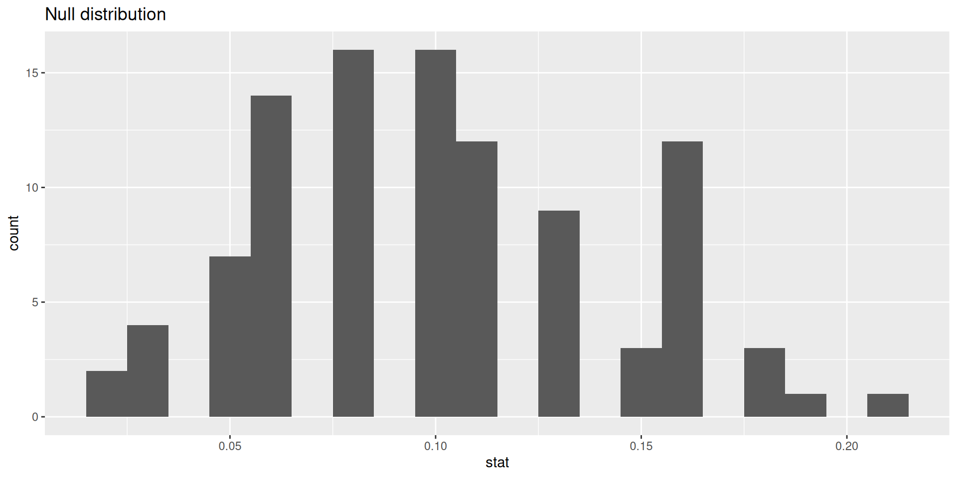
p-value

Calculating the p-value, visually

What is the p-value: How often was the simulated sample proportion at least as extreme as the observed sample proportion?¹

ggplot(data = null_dist, mapping = aes(x = stat)) +
  geom_histogram(binwidth = 0.01) +
  labs(title = "Null distribution")  +
 geom_vline(xintercept = 3/62, color = "red")

1. This a one-sided hypothesis test because we are looking for extremely lower rates not also extremely higher rates. We do one-sided test if we know the direction of interest, here “low” and “lower” rates.

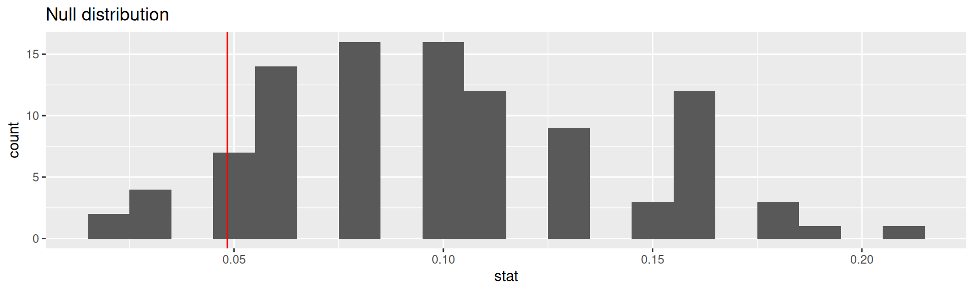
Calculating the p-value, directly

null_dist |>
 summarise(p_value = sum(stat <= 3/62)/n())

# A tibble: 1 × 1
  p_value
    <dbl>
1    0.13

This is the fraction of simulations where complications was equal or below 0.0483871.

Significance level

• A significance level \(\alpha\) is a threshold we make up to make our judgment about the plausibility of the null hypothesis being true given the observed data.

• We often use \(\alpha = 0.05 = 5\%\) as the cutoff for whether the p-value is low enough that the data are unlikely to have come from the null model.

• If p-value < \(\alpha\), reject \(H_0\) in favor of \(H_A\): The data provide convincing evidence for the alternative hypothesis.

• If p-value > \(\alpha\), fail to reject \(H_0\) in favor of \(H_A\): The data do not provide convincing evidence for the alternative hypothesis.

What is the conclusion of the hypothesis test?

Since the p-value is greater than the significance level, we fail to reject the null hypothesis. These data do not provide convincing evidence that this consultant incurs a lower complication rate than the 10% overall US complication rate.

100 simulations is not sufficient

• We simulate 15,000 times to get an accurate distribution.

null_dist <- organ_donor |>
  specify(response = outcome, success = "complication") |>
  hypothesize(null = "point", 
              p = c("complication" = 0.10, "no complication" = 0.90)) |> 
  generate(reps = 15000, type = "simulate") |> 
  calculate(stat = "prop")
ggplot(data = null_dist, mapping = aes(x = stat)) +
  geom_histogram(binwidth = 0.01) +
  geom_vline(xintercept = 3/62, color = "red")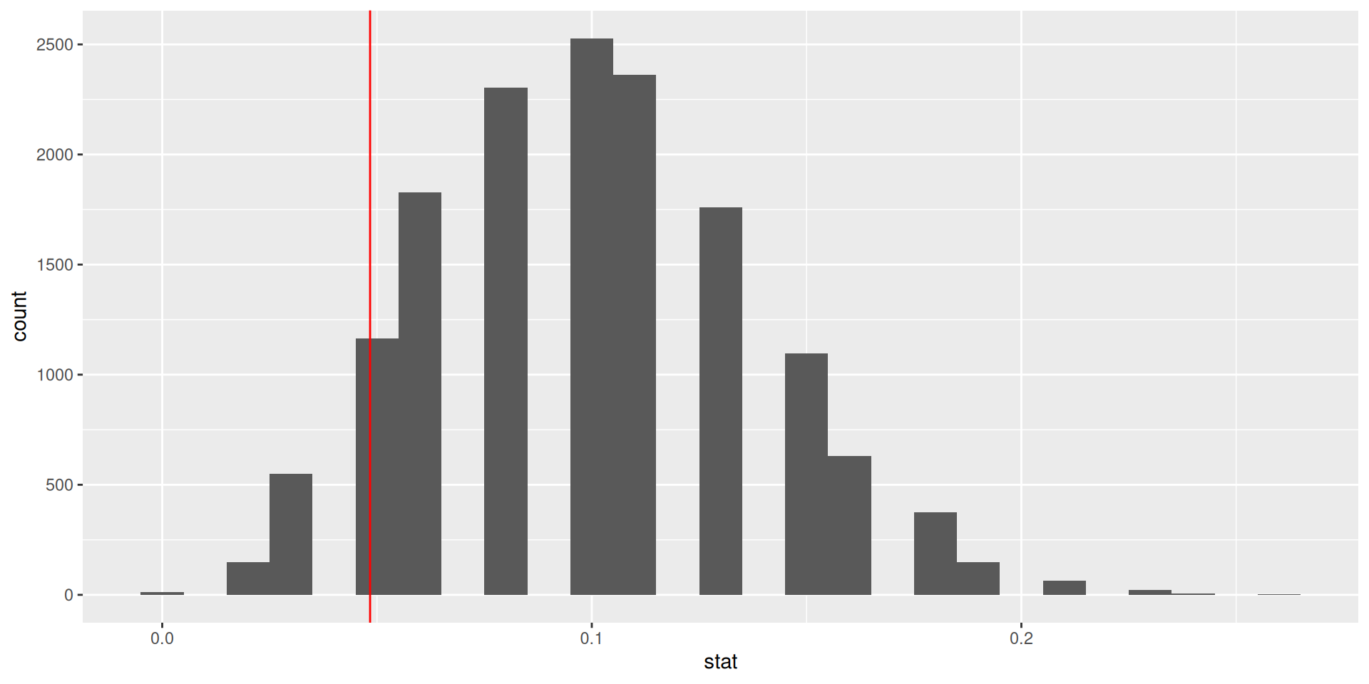

Our more robust p-value

For the null distribution with 15,000 simulations

null_dist |>
  filter(stat <= 3/62) |>
  summarise(p_value = n()/nrow(null_dist))

# A tibble: 1 × 1
  p_value
    <dbl>
1   0.125

Oh OK, our first p-value was much more borderline in favor of the alternative hypothesis.

p-value in model outputs

Model output for a linear model with palmer penguins.

linear_reg() |> set_engine("lm") |> 
    fit(bill_length_mm ~ bill_depth_mm, data = penguins) |> tidy()

# A tibble: 2 × 5
  term          estimate std.error statistic  p.value
  <chr>            <dbl>     <dbl>     <dbl>    <dbl>
1 (Intercept)     55.1       2.52      21.9  6.91e-67
2 bill_depth_mm   -0.650     0.146     -4.46 1.12e- 5

Model output for a logistic regression model with email from openintro

logistic_reg() |>  set_engine("glm") |>
  fit(spam ~ from + cc, data = email, family = "binomial") |> tidy()

# A tibble: 3 × 5
  term         estimate std.error statistic p.value
  <chr>           <dbl>     <dbl>     <dbl>   <dbl>
1 (Intercept)  13.6      309.        0.0439   0.965
2 from1       -15.8      309.       -0.0513   0.959
3 cc            0.00423    0.0193    0.220    0.826

What do the p-values mean? What is the null hypothesis?

Null-Hypothesis: There is no relationship between the predictor variable and the response variable, that means that the coefficient is equal to zero.

Smaller p-value \(\to\) more evidence for rejecting the hypothesis that there is no effect.

xkcd on p-values

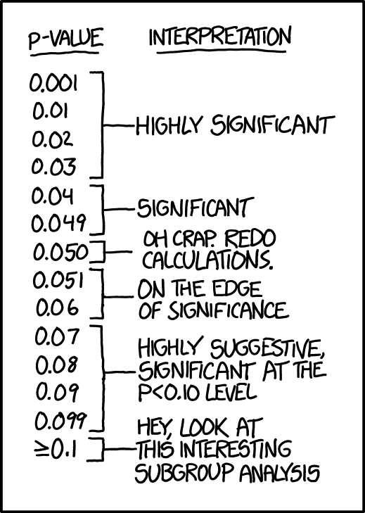
• Significance levels are fairly arbitrary. Sometimes they are used (wrongly) as definitive judgments
• They can even be used to do p-hacking: Searching for “significant” effects in observational data
• In parts of science it has become a “gamed” performance metric.
• The p-value says nothing about effect size!

p-value misinterpretation

p-values do not measure¹

• the probability that the studied hypothesis is true
• the probability that the data were produced by random chance alone
• the size of an effect
• the “importance of a result” or “evidence regarding a model or hypothesis” (it is only against the null hypothesis).

Correct:
The p-value is the probability of obtaining test results at least as extreme as the result actually observed, under the assumption that the null hypothesis is correct.

p-values and significance tests, when properly applied and interpreted, increase the rigor of the conclusions drawn from data.²

1. From the American Statistical Association (ASA) 2016

2. From the American Statistical Association (ASA) 2019

Classification: Compare logistic regression and decision tree

Purpose of the section

• Go again through the modeling workflow (with tidymodels) and see that large parts are identical
• Look again at the coefficients of a logistic regression model
• Learn the basic idea of a decision tree (you will not learn the details here)
• Do the classification with both models and compare the confusion matrices

Specify recipe and models

For both logistic regression and decision tree:

peng_recipe <- recipe(sex ~ ., data = penguins) |> 
 step_rm(year)

• We specify a recipe to predict sex with all available variables in penguins
  • In typical model development, more pre-processing steps are done.

Logistic Regression

peng_logreg <- logistic_reg() |>
 set_engine("glm")

peng_logreg specifies to fit with glm (generalized linear model from base R)

Decision Tree

peng_tree <- decision_tree() |>
 set_engine("rpart") |>
 set_mode("classification")

peng_tree specifies to fit for classification with the rpart¹ as engine.

1. rpart is a package for recursive partitioning and regression trees. Different decision tree procedures are subsumed as classification and regression trees (CART)

Split and fit

For logistic regression and decision tree:

Split into test and training data

set.seed(1)
penguins_split <- initial_split(penguins, prop = 0.7, strata = sex)
peng_train <- training(penguins_split)
peng_test <- testing(penguins_split)
peng_workflow <- workflow() |> add_recipe(peng_recipe)

Logistic Regression

peng_logreg_fit <- peng_workflow |> 
 add_model(peng_logreg) |> 
 fit(data = peng_train)

Decision Tree

peng_tree_fit <- peng_workflow |> 
 add_model(peng_tree) |> 
 fit(data = peng_train)

Look at fitted logistic regression

peng_logreg_fit |> tidy()

# A tibble: 9 × 5
  term               estimate std.error statistic      p.value
  <chr>                 <dbl>     <dbl>     <dbl>        <dbl>
1 (Intercept)       -90.4      16.7        -5.41  0.0000000632
2 speciesChinstrap   -6.06      1.90       -3.19  0.00142     
3 speciesGentoo      -8.65      3.49       -2.48  0.0132      
4 islandDream         0.752     1.15        0.656 0.512       
5 islandTorgersen     0.380     1.13        0.335 0.737       
6 bill_length_mm      0.532     0.150       3.56  0.000378    
7 bill_depth_mm       1.79      0.456       3.93  0.0000866   
8 flipper_length_mm   0.0552    0.0620      0.891 0.373       
9 body_mass_g         0.00693   0.00162     4.27  0.0000193   

• What do the categorical predictors tell us? Which are signigficant?
• What do the numerical predictors tell us? Which are signigficant?
• Why is the coefficient for body_mass_g so small, but highly significant?

Categorical predictors: We have 3 species, 3 island. So, we see 4 new variables, 2 for species and 2 for island (the third is the reference category). Species are significant (p < 0.05), but islands not.

Numerical predictors: flipper_length_mm is insignificant, though its coefficient is larger than for body_mass_g. Reason: values of body_mass_g are larger than those of flipper_length_mm. Body mass differs by much more grams than flipper length differs by millimeters.

What is a decision tree?

peng_tree_fit

══ Workflow [trained] ══════════════════════════════════════════════════════════
Preprocessor: Recipe
Model: decision_tree()

── Preprocessor ────────────────────────────────────────────────────────────────
1 Recipe Step

• step_rm()

── Model ───────────────────────────────────────────────────────────────────────
n=234 (6 observations deleted due to missingness)

node), split, n, loss, yval, (yprob)
      * denotes terminal node

 1) root 234 117 female (0.50000000 0.50000000)  
   2) bill_length_mm< 48.15 166  57 female (0.65662651 0.34337349)  
     4) bill_depth_mm< 18.05 103  14 female (0.86407767 0.13592233)  
       8) body_mass_g< 4987.5 88   4 female (0.95454545 0.04545455) *
       9) body_mass_g>=4987.5 15   5 male (0.33333333 0.66666667) *
     5) bill_depth_mm>=18.05 63  20 male (0.31746032 0.68253968)  
      10) body_mass_g< 3875 29  10 female (0.65517241 0.34482759)  
        20) flipper_length_mm< 190.5 18   3 female (0.83333333 0.16666667) *
        21) flipper_length_mm>=190.5 11   4 male (0.36363636 0.63636364) *
      11) body_mass_g>=3875 34   1 male (0.02941176 0.97058824) *
   3) bill_length_mm>=48.15 68   8 male (0.11764706 0.88235294)  
     6) body_mass_g< 5175 35   8 male (0.22857143 0.77142857)  
      12) bill_depth_mm< 18 9   3 female (0.66666667 0.33333333) *
      13) bill_depth_mm>=18 26   2 male (0.07692308 0.92307692) *
     7) body_mass_g>=5175 33   0 male (0.00000000 1.00000000) *

• A sequence of rules for yes/no decisions
• Selects variables and thresholds which separate the data to predict (here sex) best
• Further details are not the scope of this course

Show rules

We “dig out” the original fitted rpart-object from the workflow-object with peng_tree_fit$fit$fit$fit and plot it:

rpart.rules(peng_tree_fit$fit$fit$fit, roundint=FALSE)

  ..y                                                                                                 
 0.05 when bill_length_mm <  48 & body_mass_g <  4988 & bill_depth_mm <  18                           
 0.17 when bill_length_mm <  48 & body_mass_g <  3875 & bill_depth_mm >= 18 & flipper_length_mm <  191
 0.33 when bill_length_mm >= 48 & body_mass_g <  5175 & bill_depth_mm <  18                           
 0.64 when bill_length_mm <  48 & body_mass_g <  3875 & bill_depth_mm >= 18 & flipper_length_mm >= 191
 0.67 when bill_length_mm <  48 & body_mass_g >= 4988 & bill_depth_mm <  18                           
 0.92 when bill_length_mm >= 48 & body_mass_g <  5175 & bill_depth_mm >= 18                           
 0.97 when bill_length_mm <  48 & body_mass_g >= 3875 & bill_depth_mm >= 18                           
 1.00 when bill_length_mm >= 48 & body_mass_g >= 5175                                                 

• The first three rules would predict female for all observations
• The last five rules would predict male for all observations

The order of male and female is because sex is a factor with the first level female and the second level male. The probabilities in front of the rule-text are for the second level: male.

Visualize tree

rpart.plot(peng_tree_fit$fit$fit$fit, 
           roundint=FALSE, tweak=1.5)

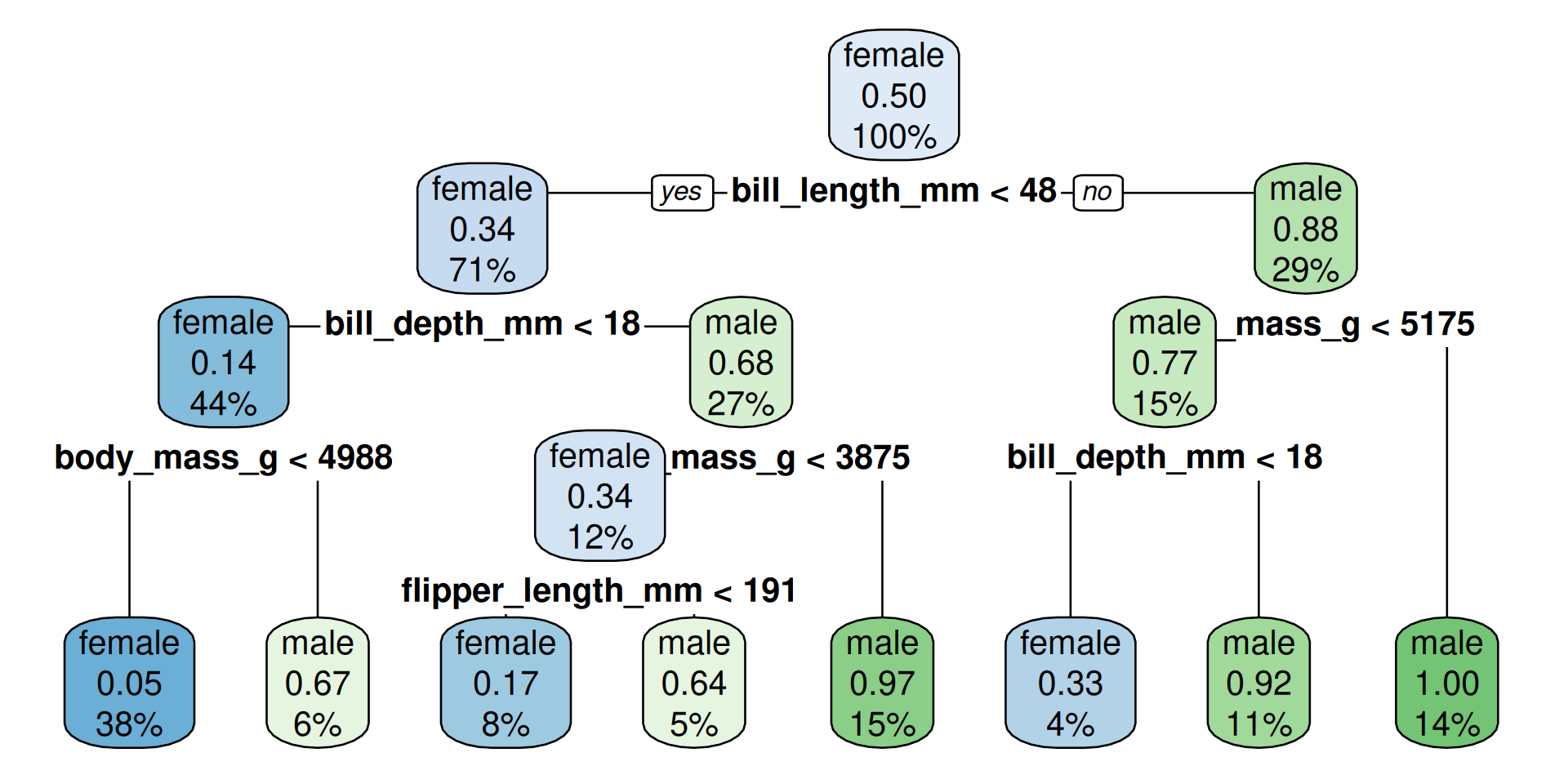
How to read?

• The percentage is the fraction of the total cases in this group
• The probability-number is the fraction of observations which are male in the group
• male of female and color would match the predicted outcome at this decision node

Make predictions for test data

peng_logreg_pred <- 
 predict(peng_logreg_fit, peng_test) |> 
 bind_cols(peng_test) 
peng_logreg_pred |> 
 conf_mat(truth = sex, estimate = .pred_class)

          Truth
Prediction female male
    female     46   10
    male        2   41

peng_tree_pred <- 
 predict(peng_tree_fit, peng_test) |> 
 bind_cols(peng_test)
peng_tree_pred |> 
 conf_mat(truth = sex, estimate = .pred_class)

          Truth
Prediction female male
    female     43   12
    male        5   39

• The logistic regression has more correct predictions.
• Warning: The function conf_mat (from yardstick of tidymodels) shows the transposed confusion matrix compared with Wikipedia:Confusion Matrix. In conf_mat, the true conditions are in columns. The wikipedia convention is that columns are the predicted conditions.

Regression: Compare linear regression and decision tree

Purpose of the section

• Go again through the modeling workflow (with tidymodels) and see that large parts are identical
• Look again at the coefficients of a linear model
• See how the decision tree looks like for a regression problem
• Compare the two most common performance measures for regression models: Root Mean Squared Error (RMSE) and R-squared

Specify recipe and models

• We specify a recipe to predict body_mass_g with all available variables in penguins and put it in a workflow
  • Typically, more pre-processing steps are specified here, but we are mostly fine

peng_recipe2 <- recipe(body_mass_g ~ ., data = penguins) |> 
 step_rm(year)
peng_workflow2 <- workflow() |> 
 add_recipe(peng_recipe2)

We can re-use the split and the training and test set.

Linear Regression

peng_linreg <- linear_reg() |>
 set_engine("lm")

Decision Tree

peng_regtree <- decision_tree() |>
 set_engine("rpart") |>
 set_mode("regression")

Fit Regression Models

Linear Regression

peng_linreg_fit <- peng_workflow2 |> 
 add_model(peng_linreg) |> 
 fit(data = peng_train)

Decision Tree

peng_regtree_fit <- peng_workflow2 |> 
 add_model(peng_regtree) |> 
 fit(data = peng_train)

Look at fitted linear regression

peng_linreg_fit |> tidy() 

# A tibble: 9 × 5
  term              estimate std.error statistic  p.value
  <chr>                <dbl>     <dbl>     <dbl>    <dbl>
1 (Intercept)         -829.     701.      -1.18  2.38e- 1
2 speciesChinstrap    -268.     109.      -2.47  1.44e- 2
3 speciesGentoo       1010.     164.       6.15  3.52e- 9
4 islandDream          -14.5     70.0     -0.208 8.36e- 1
5 islandTorgersen      -21.4     75.7     -0.283 7.77e- 1
6 bill_length_mm        19.8      8.55     2.32  2.13e- 2
7 bill_depth_mm         53.7     23.9      2.25  2.56e- 2
8 flipper_length_mm     13.6      3.54     3.84  1.58e- 4
9 sexmale              393.      58.5      6.71  1.57e-10

• What do the categorical predictors tell us? Which are signigficant?
• What do the numerical predictors tell us? Which are signigficant?

Categorical predictors: We have 3 species, 3 island and 2 sex. So, we see 5 new variables. Species and sex are significant, but islands not.

Numerical predictors: All 3 are significant.

Show rules

rpart.rules(peng_regtree_fit$fit$fit$fit, roundint=FALSE)

  ..y                                                    
 3418 when species is Adelie or Chinstrap & sex is female
 3961 when species is Adelie or Chinstrap & sex is   male
 4693 when species is              Gentoo & sex is female
 5474 when species is              Gentoo & sex is   male

• For each terminal node a certain value is predicted (the mean of the remaining penguins)

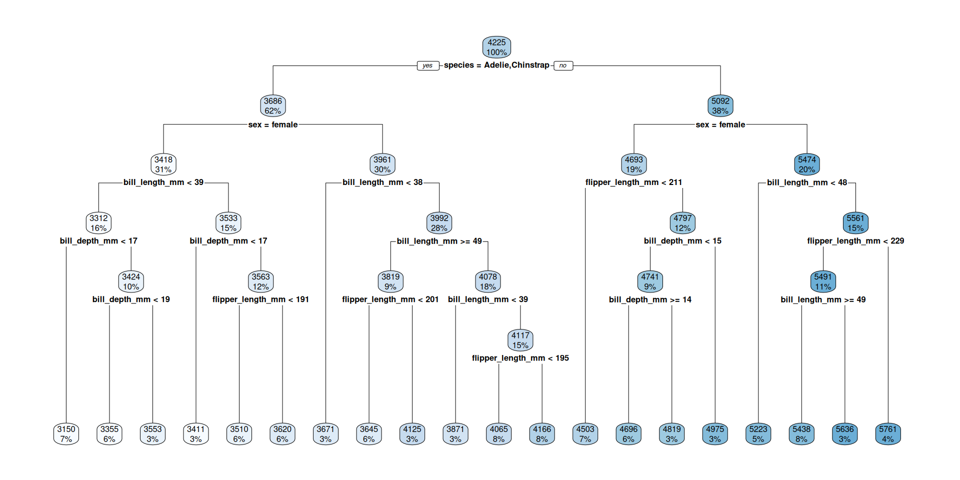
Visualize tree

rpart.plot(peng_regtree_fit$fit$fit$fit, 
           roundint=FALSE, tweak=1.5)

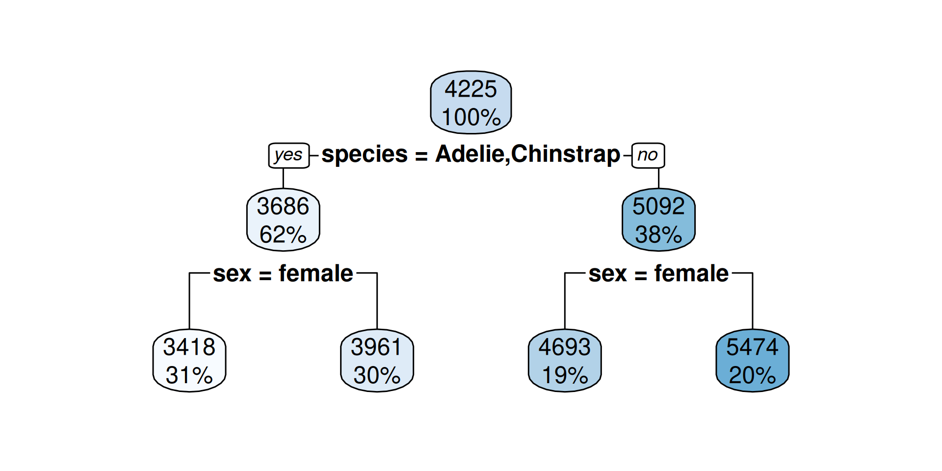
How to read?

• The percentage is the fraction of the total cases in this group
• The number is the predicted outcome (mean body mass) at this decision node

Make predictions for test data

Linear Regression

peng_linreg_pred <- 
 predict(peng_linreg_fit, peng_test) |> 
 bind_cols(peng_test) 
peng_linreg_pred |> 
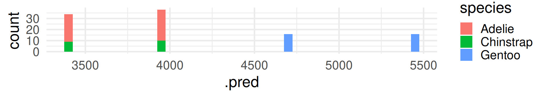
 select(.pred, body_mass_g, everything()) |> 
 slice(10*(1:10)) # show selected rows

# A tibble: 10 × 9
   .pred body_mass_g species   island    bill_length_mm bill_depth_mm
   <dbl>       <int> <fct>     <fct>              <dbl>         <dbl>
 1 3349.        3700 Adelie    Torgersen           36.6          17.8
 2 3979.        3950 Adelie    Dream               38.8          20  
 3 3902.        3800 Adelie    Dream               36.3          19.5
 4 4106.        3875 Adelie    Torgersen           41.4          18.5
 5 3499.        3400 Adelie    Dream               40.2          17.1
 6 4597.        4150 Gentoo    Biscoe              42            13.5
 7 4688.        4200 Gentoo    Biscoe              45.5          13.9
 8 4929.        4850 Gentoo    Biscoe              48.5          15  
 9 4014.        4150 Chinstrap Dream               52            19  
10 4108.        4050 Chinstrap Dream               50.7          19.7
# ℹ 3 more variables: flipper_length_mm <int>, sex <fct>, year <int>

Decision Tree

peng_regtree_pred <- 
 predict(peng_regtree_fit, peng_test) |> 
 bind_cols(peng_test)
peng_regtree_pred |> 
 select(.pred, body_mass_g, species, sex) |> 
 slice(10*(1:10)) # show same selected rows

# A tibble: 10 × 4
   .pred body_mass_g species   sex   
   <dbl>       <int> <fct>     <fct> 
 1 3418         3700 Adelie    female
 2 3961.        3950 Adelie    male  
 3 3961.        3800 Adelie    male  
 4 3961.        3875 Adelie    male  
 5 3418         3400 Adelie    female
 6 4693.        4150 Gentoo    female
 7 4693.        4200 Gentoo    female
 8 4693.        4850 Gentoo    female
 9 3961.        4150 Chinstrap male  
10 3961.        4050 Chinstrap male  

Regression Performance Evaluation

R-squared: Percentage of variability in body_mass_g explained by the model

Linear Regression

rsq(peng_linreg_pred, 
    truth = body_mass_g, estimate = .pred)

# A tibble: 1 × 3
  .metric .estimator .estimate
  <chr>   <chr>          <dbl>
1 rsq     standard       0.861

Decision Tree

rsq(peng_regtree_pred, 
    truth = body_mass_g, estimate = .pred)

# A tibble: 1 × 3
  .metric .estimator .estimate
  <chr>   <chr>          <dbl>
1 rsq     standard       0.806

Root Mean Squared Error (RMSE): \(\text{RMSE} = \sqrt{\frac{1}{n}\sum_{i = 1}^n (y_i - \hat{y}_i)^2}\)
where \(\hat{y}_i\) is the predicted value and \(y_i\) the true value. (The name RMSE is descriptive.)

rmse(peng_linreg_pred, 
     truth = body_mass_g, 
     estimate = .pred)

# A tibble: 1 × 3
  .metric .estimator .estimate
  <chr>   <chr>          <dbl>
1 rmse    standard        290.

rmse(peng_regtree_pred, 
     truth = body_mass_g, 
     estimate = .pred)

# A tibble: 1 × 3
  .metric .estimator .estimate
  <chr>   <chr>          <dbl>
1 rmse    standard        337.

Which model is better in prediction? Linear regression. The R-squared is higher.

What RMSE is better?

Lower. The lower the error, the better the model’s prediction.

It is the other way round than R-squared! Do not confuse them.

Notes:

• The common method to fit a linear model is the ordinary least squares (OLS) method
• That means the fitted parameters should deliver the lowest possible sum of squared errors (SSE) between predicted and observed values.
• Minimizing the sum of squared errors (SSE) is identical to minimizing the mean of squared errors (MSE) because it only adds the factor \(1/n\).
• Minimizing the mean of squared errors (MSE) is identical to minimizing the root mean of squared errors (RMSE) because the square root is strictly monotone function.

Conclusion: RMSE can be seen as a definition of the OLS optimization goal.

Interpreting RMSE

In contrast to R-squared, RMSE can only be interpreted with knowledge about the range and of the response variable! It also has the same unit (grams for body_mass_g).

peng_test |> 
 ggplot(aes(x=body_mass_g, fill = species)) + 
 geom_histogram(binwidth = 50) + 
 theme_minimal(base_size = 20)

peng_linreg_pred |> 
 ggplot(aes(x=.pred, fill = species)) + 
 geom_histogram(binwidth = 50) + 
 theme_minimal(base_size = 20)

peng_regtree_pred |> 
 ggplot(aes(x=.pred, fill = species)) + 
 geom_histogram(binwidth = 50) + 
 theme_minimal(base_size = 20)

The RMSE shows many grams predicted values deviate from the true value on average. (Taking the squaring of differences and root of the average into account.)

Overfitting with decision trees

Compare training and test data

Linear Regression Predict with test data:

predict(peng_linreg_fit, peng_test) |> bind_cols(peng_test) |> 
 metrics(truth = body_mass_g, estimate = .pred) |> slice(1:2)

# A tibble: 2 × 3
  .metric .estimator .estimate
  <chr>   <chr>          <dbl>
1 rmse    standard     290.   
2 rsq     standard       0.861

Predict with training data:

predict(peng_linreg_fit, peng_train) |> bind_cols(peng_train) |> 
 metrics(truth = body_mass_g, estimate = .pred) |> slice(1:2)

# A tibble: 2 × 3
  .metric .estimator .estimate
  <chr>   <chr>          <dbl>
1 rmse    standard     283.   
2 rsq     standard       0.880

Decision Tree Predict with test data:

predict(peng_regtree_fit, peng_test) |> bind_cols(peng_test) |> 
 metrics(truth = body_mass_g, estimate = .pred) |> slice(1:2)

# A tibble: 2 × 3
  .metric .estimator .estimate
  <chr>   <chr>          <dbl>
1 rmse    standard     337.   
2 rsq     standard       0.806

Predict with training data:

predict(peng_regtree_fit, peng_train) |> bind_cols(peng_train) |> 
 metrics(truth = body_mass_g, estimate = .pred) |> slice(1:2)

# A tibble: 2 × 3
  .metric .estimator .estimate
  <chr>   <chr>          <dbl>
1 rmse    standard     309.   
2 rsq     standard       0.857

Where is the prediction better? (Lower RMSE, higher R-squared)

Performance is better for training data (compare values to testing data of the same model). Why? It was used to fit. The model is optimized to predict the training data.

Make a deeper tree

• In decision_tree() we can set the maximal depth of the tree to 30.
  
• The trees we had before were also automatically pruned by sensible defaults.
  
• By setting the cost complexity parameter to -1 we avoid pruning.¹

peng_regtree_deep <- decision_tree(
 cost_complexity = -1,
 tree_depth = 30
) |>
 set_engine("rpart") |>
 set_mode("regression")
peng_regtree_deep_fit <- peng_workflow2 |> add_model(peng_regtree_deep) |> 
 fit(data = peng_train)

1. The details of this go beyond the scope of this course.

The deep tree

Compare pruned and deep tree

Pruned decision tree

Predict with training data:

peng_regtree_fit |> 
 predict(new_data = peng_train) |> bind_cols(peng_train) |> 
 metrics(truth = body_mass_g, estimate = .pred) |> slice(1:2)

# A tibble: 2 × 3
  .metric .estimator .estimate
  <chr>   <chr>          <dbl>
1 rmse    standard     309.   
2 rsq     standard       0.857

Predict with testing data:

peng_regtree_fit |> 
 predict(peng_test) |> bind_cols(peng_test) |> 
 metrics(truth = body_mass_g, estimate = .pred) |> slice(1:2)

# A tibble: 2 × 3
  .metric .estimator .estimate
  <chr>   <chr>          <dbl>
1 rmse    standard     337.   
2 rsq     standard       0.806

Deep decision tree

Predict with training data:

peng_regtree_deep_fit |> 
 predict(new_data = peng_train) |> bind_cols(peng_train) |> 
 metrics(truth = body_mass_g, estimate = .pred) |> slice(1:2)

# A tibble: 2 × 3
  .metric .estimator .estimate
  <chr>   <chr>          <dbl>
1 rmse    standard     247.   
2 rsq     standard       0.908

Predict with testing data:

peng_regtree_deep_fit |> 
 predict(peng_test) |> bind_cols(peng_test) |> 
 metrics(truth = body_mass_g, estimate = .pred) |> slice(1:2)

# A tibble: 2 × 3
  .metric .estimator .estimate
  <chr>   <chr>          <dbl>
1 rmse    standard     333.   
2 rsq     standard       0.808

More in an R-script

• Overfitting in spam predicton models.

• From decision trees to random forrests.

Move to the script.

What do we mean by “model”? How to be specific

“Model” in Statistical Learning

We already had the difference between variable-based and agent-based models in earlier lectures.

But even in the variable-based model setting of statistical learning, the term model can be more or less abstract:

1. Very general: \(Y = f(X_1, \dots, X_m) + \varepsilon\) where \(Y\) is the response variable and \(X_i\) are features which we put in our model: the abstract and unknown function \(f\).
   \(\varepsilon\) is the error which we can never explain usually do not know.
2. More specific: The model \(f\) could already be of a specific type, like logistic regression, a decision tree or other functional forms. As this need not be the real function we may call it assumed model \(\hat f\) For example a linear model \(\hat f(X_1, \dots, X_m) = \beta_0 + \beta_1 X_1 + \dots + \beta_m X_m + \varepsilon\). Now, the model has specified parameters which values are unknown.

More specific: Fitted model

3. Fitted model: When we have a data set with values for \(Y, X_1, \dots, X_m\) we can fit values for the parameters \(\hat\beta_0, \dots, \hat\beta_m\) to the data. This is the fitted model \(\hat f\). This is called parameter estimation: We estimate \(\hat\beta_0, \dots, \hat\beta_m\) with the hope that they match the real values \(\beta_0, \dots, \beta_m\) and that the linear model \(\hat f\) matches the real function \(f\).
4. Now we could specify further to fit a specific parameterized model with a specific algorithm, and a specific set of hyperparameters, and maybe more …

Sometimes model means only a certain aspect of all these, for example the formula like sex ~ bill_length_mm + bill_depth_mm + flipper_length_mm + body_mass_g + species + island

Take away: “Model” can mean things with very different granularity. That is OK because they are all related and all fit the definition of being a simplified representation of reality.

Be prepared to specify what you mean when you are talking about a model.