Isn’t that a data frame? No.
Note: A matrix can also be of characters or logicals, it can also have row- and column-names.
The elements1 of an \(m\)-by-\(n\) matrix \(A\)
![]()
A matrix can be interpreted
In R and python, a vector is not specified as row or columns. In matrix terminology a
column vector is a \(m\)-by-1 matrix \(\left[\begin{array}{c} a_{1} \\ \vdots \\ a_{m}\end{array}\right]\)
row vector is a 1-by-\(n\) matrix \(\left[\begin{array}{c} a_{1}\ \cdots\ a_{n}\end{array}\right]\)
Convention: If a vector is not specified as row or column it is usually treated as columns if that is relevant.
t() transposesThink vectorized!
![]()
(In the graphic \(x\cdot y\) stands for \(x^Ty\))
Think of palmer penguins dummy variables
| ID | sex male | species Chinstrap | species Gentoo |
|---|---|---|---|
| 1 | 0 | 1 | 0 |
| 2 | 0 | 1 | 0 |
| 3 | 0 | 0 | 1 |
| 4 | 1 | 0 | 1 |
| 5 | 1 | 0 | 0 |
| 6 | 1 | 0 | 0 |
| 7 | 1 | 1 | 0 |
This is the equation of a model:
average flipper_length_mm \(= \beta_0 + \beta_1\cdot\) body_mass_g \(+ \beta_2\cdot\) bill_length_mm $ + _3$ bill_length_mm
More mathy renamed: \(Y = \beta_0 + \beta_1X_1+ \beta_2X_2 + \beta_3X_3+ \varepsilon\)
We also add \(\varepsilon\) as the unknown error the model cannot capture. (So, we do not need to write “average” \(Y\))
For matrix description we join \(X_1\), \(X_2\), and \(X3\) as columns in the matrix \(X\) and put a matrix of ones as \(X_0\) for the intercept as another column, and the intercept \(\beta_0\) and the coefficients \(\beta_1\), \(\beta_2\), and \(\beta_3\) into a vector \(\beta\).
The matrix form: \(Y = X\cdot\beta + \varepsilon\)
penguins <- na.omit(penguins)
peng_fit <- linear_reg() |>
set_engine("lm") |>
fit(flipper_length_mm ~ body_mass_g + bill_length_mm + bill_depth_mm, data = penguins)
beta <- peng_fit$fit$coefficients
beta (Intercept) body_mass_g bill_length_mm bill_depth_mm
156.78217410 0.01096719 0.58843506 -1.62201792
X <- penguins |>
select(body_mass_g, bill_length_mm, bill_depth_mm) |>
mutate(intercept = 1) |> # We add a column of ones for the intercept
select(intercept, everything()) |>
as.matrix()
Y <- matrix(penguins$flipper_length_mm, ncol = 1)
# These are our predictions in computed in matrix language
X %*% beta [,1]
[1,] 190.5852
[2,] 193.4776
[3,] 186.9432
[4,] 184.9096
[5,] 186.5244
[6,] 190.5565
[7,] 199.3289
[8,] 187.5144
[9,] 186.7843
[10,] 191.1731
[11,] 190.0256
[12,] 186.5731
[13,] 197.5673
[14,] 183.6451
[15,] 195.0390
[16,] 186.6305
[17,] 188.1163
[18,] 188.4396
[19,] 193.2223
[20,] 193.3901
[21,] 188.5731
[22,] 189.4366
[23,] 186.6747
[24,] 183.4610
[25,] 193.2781
[26,] 188.5810
[27,] 192.0855
[28,] 187.3452
[29,] 192.9651
[30,] 187.0928
[31,] 191.1381
[32,] 190.4935
[33,] 190.5403
[34,] 183.7941
[35,] 200.2188
[36,] 183.6104
[37,] 193.7173
[38,] 181.9568
[39,] 199.0341
[40,] 184.0437
[41,] 200.0394
[42,] 187.7112
[43,] 186.7685
[44,] 192.8001
[45,] 189.7597
[46,] 196.8812
[47,] 186.1801
[48,] 194.2842
[49,] 179.5295
[50,] 191.5525
[51,] 190.2794
[52,] 191.8540
[53,] 182.5911
[54,] 189.0538
[55,] 184.9239
[56,] 195.1156
[57,] 190.8149
[58,] 195.8633
[59,] 181.7212
[60,] 195.3852
[61,] 188.1350
[62,] 194.9518
[63,] 184.4314
[64,] 198.7156
[65,] 185.1583
[66,] 193.0700
[67,] 191.1190
[68,] 198.5902
[69,] 189.8649
[70,] 198.5704
[71,] 194.1779
[72,] 189.9769
[73,] 190.9026
[74,] 194.4435
[75,] 184.3383
[76,] 205.0243
[77,] 189.5591
[78,] 192.0313
[79,] 186.5990
[80,] 187.0911
[81,] 188.1884
[82,] 186.7111
[83,] 191.4969
[84,] 188.6603
[85,] 187.5265
[86,] 198.7673
[87,] 186.3409
[88,] 199.5297
[89,] 186.2144
[90,] 197.2931
[91,] 189.6106
[92,] 198.1961
[93,] 181.9497
[94,] 197.1607
[95,] 189.1961
[96,] 200.2876
[97,] 186.7380
[98,] 193.1952
[99,] 180.9934
[100,] 188.4204
[101,] 192.7240
[102,] 189.5921
[103,] 186.4481
[104,] 203.7526
[105,] 194.3878
[106,] 201.1369
[107,] 186.5283
[108,] 196.8695
[109,] 189.2805
[110,] 196.9167
[111,] 183.7263
[112,] 186.8806
[113,] 186.9551
[114,] 187.2632
[115,] 184.7315
[116,] 185.2354
[117,] 190.6998
[118,] 193.6339
[119,] 185.1549
[120,] 193.7231
[121,] 186.9835
[122,] 198.6782
[123,] 185.4446
[124,] 197.4046
[125,] 186.8687
[126,] 189.3862
[127,] 186.8144
[128,] 197.9193
[129,] 188.2167
[130,] 195.3536
[131,] 184.1660
[132,] 191.4293
[133,] 189.0794
[134,] 197.7195
[135,] 189.9892
[136,] 190.8849
[137,] 183.9796
[138,] 194.0100
[139,] 184.3825
[140,] 189.4297
[141,] 196.2899
[142,] 186.5848
[143,] 186.9307
[144,] 190.7935
[145,] 190.8079
[146,] 195.0637
[147,] 211.8508
[148,] 222.2780
[149,] 211.3725
[150,] 224.0623
[151,] 220.4953
[152,] 212.1479
[153,] 212.4582
[154,] 216.4746
[155,] 208.7820
[156,] 215.8229
[157,] 209.6250
[158,] 220.3689
[159,] 212.3318
[160,] 225.7391
[161,] 206.1133
[162,] 224.4844
[163,] 205.1131
[164,] 230.1718
[165,] 213.0911
[166,] 219.6210
[167,] 225.6398
[168,] 214.6373
[169,] 208.8808
[170,] 213.7832
[171,] 215.6136
[172,] 215.3492
[173,] 222.5437
[174,] 212.3990
[175,] 222.2550
[176,] 217.3760
[177,] 210.4804
[178,] 215.1857
[179,] 230.6301
[180,] 218.1495
[181,] 218.0464
[182,] 213.9155
[183,] 212.4255
[184,] 208.3212
[185,] 218.6478
[186,] 203.0071
[187,] 222.5293
[188,] 208.3756
[189,] 213.7325
[190,] 221.5760
[191,] 213.6311
[192,] 207.0721
[193,] 219.9309
[194,] 217.5628
[195,] 215.8777
[196,] 214.3615
[197,] 220.5769
[198,] 208.2192
[199,] 216.7685
[200,] 214.5266
[201,] 213.6670
[202,] 207.1685
[203,] 214.0617
[204,] 207.4873
[205,] 222.4904
[206,] 207.1166
[207,] 217.9259
[208,] 209.3833
[209,] 225.2332
[210,] 212.2457
[211,] 221.3493
[212,] 223.2427
[213,] 210.8923
[214,] 223.1535
[215,] 212.6144
[216,] 213.6180
[217,] 215.7740
[218,] 217.1679
[219,] 211.3011
[220,] 223.0376
[221,] 212.1493
[222,] 226.2155
[223,] 213.0898
[224,] 222.0331
[225,] 212.8783
[226,] 222.1427
[227,] 212.8125
[228,] 219.0883
[229,] 212.9132
[230,] 220.0300
[231,] 209.4123
[232,] 222.0624
[233,] 215.4897
[234,] 220.7333
[235,] 214.6902
[236,] 218.9848
[237,] 212.1309
[238,] 221.7599
[239,] 212.3148
[240,] 218.2384
[241,] 214.2364
[242,] 214.1634
[243,] 212.6286
[244,] 217.6657
[245,] 214.1819
[246,] 223.5177
[247,] 213.9768
[248,] 221.6636
[249,] 218.5260
[250,] 209.0221
[251,] 222.8963
[252,] 209.7281
[253,] 220.9130
[254,] 216.6794
[255,] 225.5510
[256,] 208.7219
[257,] 220.9673
[258,] 209.0789
[259,] 227.4107
[260,] 225.0243
[261,] 216.3481
[262,] 214.3170
[263,] 224.0350
[264,] 216.4030
[265,] 219.2534
[266,] 193.4955
[267,] 197.3466
[268,] 195.8564
[269,] 191.8247
[270,] 196.5295
[271,] 197.8279
[272,] 190.0317
[273,] 198.5751
[274,] 198.7079
[275,] 195.2694
[276,] 197.0067
[277,] 195.6785
[278,] 196.9563
[279,] 202.4394
[280,] 195.2626
[281,] 199.1237
[282,] 190.1318
[283,] 202.6181
[284,] 191.7528
[285,] 204.4681
[286,] 193.1528
[287,] 194.2244
[288,] 187.0819
[289,] 196.7652
[290,] 191.4197
[291,] 202.0763
[292,] 193.9415
[293,] 196.7667
[294,] 195.7923
[295,] 205.3119
[296,] 189.0187
[297,] 202.0963
[298,] 191.4431
[299,] 201.2639
[300,] 195.3398
[301,] 200.2550
[302,] 197.3325
[303,] 206.4476
[304,] 187.0657
[305,] 205.3377
[306,] 197.3066
[307,] 195.6128
[308,] 194.6865
[309,] 194.3668
[310,] 198.0038
[311,] 205.4714
[312,] 194.5171
[313,] 200.9829
[314,] 192.3982
[315,] 198.3298
[316,] 194.9507
[317,] 199.5298
[318,] 195.0946
[319,] 199.0792
[320,] 190.4699
[321,] 194.8414
[322,] 192.0973
[323,] 197.9310
[324,] 197.5030
[325,] 190.8070
[326,] 199.0130
[327,] 197.5879
[328,] 196.1296
[329,] 201.3697
[330,] 190.3090
[331,] 197.8490
[332,] 200.8218
[333,] 197.3910
1 2 3 4 5 6 7 8
190.5852 193.4776 186.9432 184.9096 186.5244 190.5565 199.3289 187.5144
9 10 11 12 13 14 15 16
186.7843 191.1731 190.0256 186.5731 197.5673 183.6451 195.0390 186.6305
17 18 19 20 21 22 23 24
188.1163 188.4396 193.2223 193.3901 188.5731 189.4366 186.6747 183.4610
25 26 27 28 29 30 31 32
193.2781 188.5810 192.0855 187.3452 192.9651 187.0928 191.1381 190.4935
33 34 35 36 37 38 39 40
190.5403 183.7941 200.2188 183.6104 193.7173 181.9568 199.0341 184.0437
41 42 43 44 45 46 47 48
200.0394 187.7112 186.7685 192.8001 189.7597 196.8812 186.1801 194.2842
49 50 51 52 53 54 55 56
179.5295 191.5525 190.2794 191.8540 182.5911 189.0538 184.9239 195.1156
57 58 59 60 61 62 63 64
190.8149 195.8633 181.7212 195.3852 188.1350 194.9518 184.4314 198.7156
65 66 67 68 69 70 71 72
185.1583 193.0700 191.1190 198.5902 189.8649 198.5704 194.1779 189.9769
73 74 75 76 77 78 79 80
190.9026 194.4435 184.3383 205.0243 189.5591 192.0313 186.5990 187.0911
81 82 83 84 85 86 87 88
188.1884 186.7111 191.4969 188.6603 187.5265 198.7673 186.3409 199.5297
89 90 91 92 93 94 95 96
186.2144 197.2931 189.6106 198.1961 181.9497 197.1607 189.1961 200.2876
97 98 99 100 101 102 103 104
186.7380 193.1952 180.9934 188.4204 192.7240 189.5921 186.4481 203.7526
105 106 107 108 109 110 111 112
194.3878 201.1369 186.5283 196.8695 189.2805 196.9167 183.7263 186.8806
113 114 115 116 117 118 119 120
186.9551 187.2632 184.7315 185.2354 190.6998 193.6339 185.1549 193.7231
121 122 123 124 125 126 127 128
186.9835 198.6782 185.4446 197.4046 186.8687 189.3862 186.8144 197.9193
129 130 131 132 133 134 135 136
188.2167 195.3536 184.1660 191.4293 189.0794 197.7195 189.9892 190.8849
137 138 139 140 141 142 143 144
183.9796 194.0100 184.3825 189.4297 196.2899 186.5848 186.9307 190.7935
145 146 147 148 149 150 151 152
190.8079 195.0637 211.8508 222.2780 211.3725 224.0623 220.4953 212.1479
153 154 155 156 157 158 159 160
212.4582 216.4746 208.7820 215.8229 209.6250 220.3689 212.3318 225.7391
161 162 163 164 165 166 167 168
206.1133 224.4844 205.1131 230.1718 213.0911 219.6210 225.6398 214.6373
169 170 171 172 173 174 175 176
208.8808 213.7832 215.6136 215.3492 222.5437 212.3990 222.2550 217.3760
177 178 179 180 181 182 183 184
210.4804 215.1857 230.6301 218.1495 218.0464 213.9155 212.4255 208.3212
185 186 187 188 189 190 191 192
218.6478 203.0071 222.5293 208.3756 213.7325 221.5760 213.6311 207.0721
193 194 195 196 197 198 199 200
219.9309 217.5628 215.8777 214.3615 220.5769 208.2192 216.7685 214.5266
201 202 203 204 205 206 207 208
213.6670 207.1685 214.0617 207.4873 222.4904 207.1166 217.9259 209.3833
209 210 211 212 213 214 215 216
225.2332 212.2457 221.3493 223.2427 210.8923 223.1535 212.6144 213.6180
217 218 219 220 221 222 223 224
215.7740 217.1679 211.3011 223.0376 212.1493 226.2155 213.0898 222.0331
225 226 227 228 229 230 231 232
212.8783 222.1427 212.8125 219.0883 212.9132 220.0300 209.4123 222.0624
233 234 235 236 237 238 239 240
215.4897 220.7333 214.6902 218.9848 212.1309 221.7599 212.3148 218.2384
241 242 243 244 245 246 247 248
214.2364 214.1634 212.6286 217.6657 214.1819 223.5177 213.9768 221.6636
249 250 251 252 253 254 255 256
218.5260 209.0221 222.8963 209.7281 220.9130 216.6794 225.5510 208.7219
257 258 259 260 261 262 263 264
220.9673 209.0789 227.4107 225.0243 216.3481 214.3170 224.0350 216.4030
265 266 267 268 269 270 271 272
219.2534 193.4955 197.3466 195.8564 191.8247 196.5295 197.8279 190.0317
273 274 275 276 277 278 279 280
198.5751 198.7079 195.2694 197.0067 195.6785 196.9563 202.4394 195.2626
281 282 283 284 285 286 287 288
199.1237 190.1318 202.6181 191.7528 204.4681 193.1528 194.2244 187.0819
289 290 291 292 293 294 295 296
196.7652 191.4197 202.0763 193.9415 196.7667 195.7923 205.3119 189.0187
297 298 299 300 301 302 303 304
202.0963 191.4431 201.2639 195.3398 200.2550 197.3325 206.4476 187.0657
305 306 307 308 309 310 311 312
205.3377 197.3066 195.6128 194.6865 194.3668 198.0038 205.4714 194.5171
313 314 315 316 317 318 319 320
200.9829 192.3982 198.3298 194.9507 199.5298 195.0946 199.0792 190.4699
321 322 323 324 325 326 327 328
194.8414 192.0973 197.9310 197.5030 190.8070 199.0130 197.5879 196.1296
329 330 331 332 333
201.3697 190.3090 197.8490 200.8218 197.3910
We do not derive it here, but as a pointer to study more relations between data manipulation and matrix thinking:
The coefficients-vector \(\beta\) has the following relation
\(X^TX \cdot \beta = X^T\cdot Y\)
This is the classical form of a systems of linear equations where we want to know \(x\) in an equation \(Ax = b\).
We can solve this in R and can compare it to the coefficients
intercept body_mass_g bill_length_mm bill_depth_mm
intercept 333.0 1400950 14649.6 5715.90
body_mass_g 1400950.0 6109136250 62493450.0 23798630.00
bill_length_mm 14649.6 62493450 654405.7 250640.99
bill_depth_mm 5715.9 23798630 250641.0 99400.11
[,1]
intercept 66922
body_mass_g 284815600
bill_length_mm 2960705
bill_depth_mm 1143413
[,1]
intercept 156.78217410
body_mass_g 0.01096719
bill_length_mm 0.58843506
bill_depth_mm -1.62201792
(Intercept) body_mass_g bill_length_mm bill_depth_mm
156.78217410 0.01096719 0.58843506 -1.62201792
In the following, we say \(S\) is the sample space which is a set of atomic events.
Example for sample spaces:
An event \(A\) is a subset of the sample space \(A \subset S\).
Important: Atomic events are events but not all events are atomic.
Two coin tosses:
For selecting one random person:
Event \(\{2,5,6\}\) = The selected person is either 2, 5, or 6.
(Not all three people which is a different random variable!)
For COVID-19 testing:
Examples
Definition: A set of all events a function \(\text{Pr}: \text{Set of all subsets of $S$} \to \mathbb{R}\) is a probability function when
This captures the essence of how we think about probabilities mathematically. Most important: We can only easily add probabilities when they do not share atomic events.
Example coin tosses: We can define a probability function \(\text{Pr}\) by assigning the same probability to each atomic event.
So, the probability one or zero HEADs is \(\text{Pr}(\{HT, TH, TT\}) = \text{Pr}(\{HT\}) + \text{Pr}(\{TH\}) + \text{Pr}(\{TT\}) = \frac{3}{4}\).
Example selection of two out of five people: We can define a probability function \(\text{Pr}\) by assigning the same probability to each atomic event.
So, the probability that 1 is among the selected \(\text{Pr}(\{12, 13, 14, 15\}) = \frac{4}{10}\).
We can compute the probabilities of all events by summing the probabilities of the atomic events in it. So, the probabilities of the atomic events are building blocks for the whole probability function.
\(\text{Pr}(\emptyset) = 0\)
For any events \(A,B \subset S\) it holds
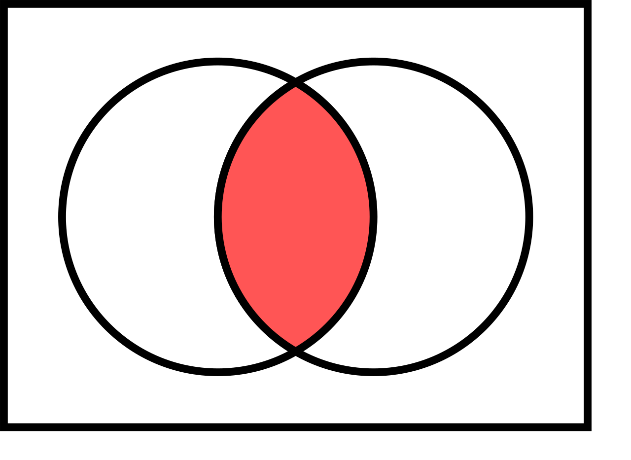
![]()
![]()
Recap from the motivation of logistic regression: When the probability of an event is \(A\) is \(\text{Pr}(A)=p\), then its odds (in favor of the event) are \(\frac{p}{1-p}\). The logistic regression model “raw” predictions are log-odds \(\log\frac{p}{1-p}\).
Definition: The conditional probability of an event \(A\) given an event \(B\) (write “\(A | B\)”) is defined as
\[\text{Pr}(A|B) = \frac{\text{Pr}(A \cap B)}{\text{Pr}(B)}\]

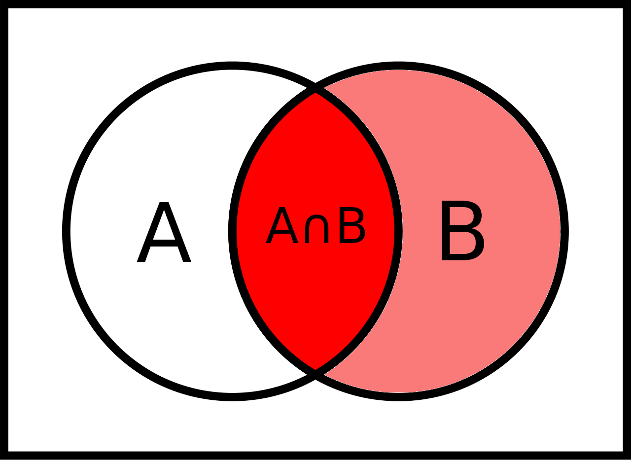
We want to know the probability of \(A\) given that we know that \(B\) has happened (or is happening for sure).
Two coin flips: \(A\) = “first coin is HEAD”, \(B\) = “one or zero HEADS in total”. What is \(\text{Pr}(A|B)\)? \(A\) = {HH, HT}, \(B\) = {TT, HT, TH} \(\to\) \(A \cap B = \{HT\}\)
\(\to\) \(\text{Pr}(A\cap B) = \frac{3}{4}\), \(\text{Pr}(A\cap B) = \frac{1}{4}\)
\(\to\) \(\text{Pr}(A|B) = \frac{1/4}{3/4} = \frac{1}{3}\)
COVID-19 Example: What is the probability that a random person in the tested sample has COVID-19 (event \(P\) “positive”) given that she has a positive test result (event \(PP\) “predicted positive”)?
\[\text{Pr}(P|PP) = \frac{\text{Pr}(P \cap PP)}{\text{Pr}(PP)}\]
Definition p-value: Probability of observed or more extreme outcome given that the null hypothesis (\(H_0\)) is true.
\[\text{p-value} = \text{Pr}(\text{observed or more extreme outcome for test-statistic} | H_0)\]
Confusion matrix of statistical classification, large version:
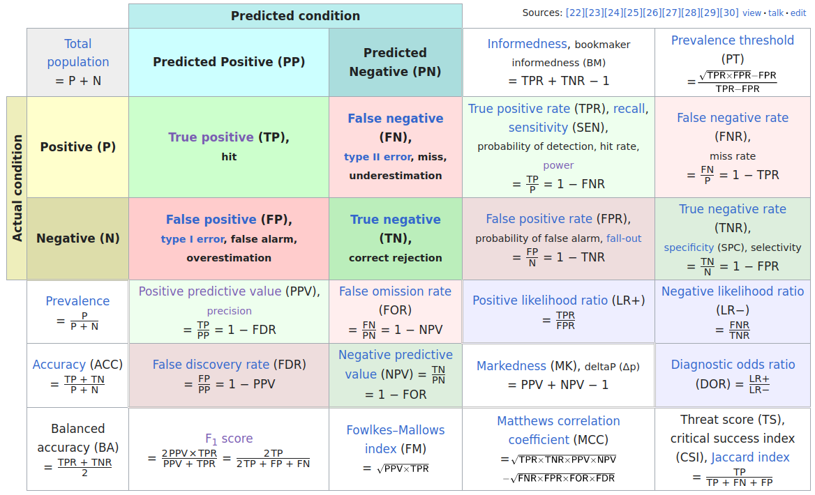
Sensitivity and Specificity
\(\to \atop \ \) Sensitivity is the true positive rate: TP / (TP + FN)
\(\ \atop \to\) Specificity is the true negative rate: TN / (TN + FP)
Positive/negative predictive value
\(\scriptsize\downarrow \ \) Positive predictive value: TP / (TP + FP)
\(\scriptsize\ \downarrow\) Negative predictive value: TN / (TN + FN)
Here TP, TN, FP, FN are the numbers of true positives, true negatives, false positives, and false negatives.
We can define fraction/probabilities for all the events \(P, N, PP, PTP, FP, FN, TN\) by dividing by \(n = TP + FP + FN + TN\).1
For example: \(\text{Pr}(TP) = \frac{TP}{n}\), \(\text{Pr}(P) = \frac{P}{n}\), \(\text{Pr}(PP) = \frac{PP}{n}\), …
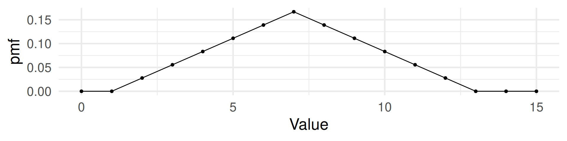
Sensitivity and specificity are conditional probabilities:
Sensitivity is the probability of a positive test result given that the person has the condition: \(\text{Pr}(PP|P) = \frac{TP}{P} = \frac{\text{Pr}(TP)}{\text{Pr}(P)}\)
Specificity is the probability of a negative test result given that the person does not have the condition: \(\text{Pr}(PN|N) = \frac{TN}{N} = \frac{\text{Pr}(TN)}{\text{Pr}(N)}\)
Positive predictive value is the probability of the condition given that the test result is positive: \(\text{Pr}(P|PP) = \frac{TP}{PP} = \frac{\text{Pr}(TP)}{\text{Pr}(PP)}\)
Negative predictive value is the probability of the condition given that the test result is negative: \(\text{Pr}(N|PN) = \frac{TN}{N} = \frac{\text{Pr}(TN)}{\text{Pr}(PN)}\)
“Flipping” conditional in positive predictive value \(\text{Pr}(P|PP)\) is sensitivity \(\text{Pr}(PP|P)\).
Positive predicted value answers the question: Given I have been tested positive, what is the probabilitiy, I have it?
Bayes’ Theorem is a fundamental theorem in probability theory that relates the conditional probabilities \(\text{Pr}(A|B)\) and \(\text{Pr}(B|A)\) to the marginal probabilities \(\text{Pr}(A)\) and \(\text{Pr}(B)\):
\[\text{Pr}(A|B) = \frac{\text{Pr}(B|A) \cdot \text{Pr}(A)}{\text{Pr}(B)}\]
Example: What is the probability that a random person in the tested sample has COVID-19 (\(P\) = positive) given that she has a positive test result (\(PP\) = predicted positive)?
\[\text{Pr}(P|PP) = \frac{\text{Pr}(PP|P) \cdot \text{Pr}(P)}{\text{Pr}(PP)}\] So, we can compute the positive predictive value \(\text{Pr}(P|PP)\) from the sensitivity \(\text{Pr}(PP|P)\) and the rate (or probability) of positive conditions \(\text{Pr}(P)\) and the rate (or probability) of positive tests \(\text{Pr}(PP)\).
\[\text{Pr}(P) = \frac{P}{n} = \frac{TP + FN}{n}\]
Sensitivity and Specificity are properties of the test (or classifier) and are independent of the prevalence of the condition in the population of interest.
The Positive/Negative Predictive Values are not!
We assume a test with sensitivity 0.9 and specificity 0.99. \(N = 1000\) people were tested.
| PP | PN | |
|---|---|---|
| P | TP | FN |
| N | FP | TN |
Sensitivity = TP / P
Specificity = TN / N
PPV = TP / PP
Prevalence = P / N
Prevalence = 0.1
\(P\) = 100 \(N\) = 900
| PP | PN | |
|---|---|---|
| P | 90 | 10 |
| N | 9 | 891 |
PPV = 90 / (90 + 9) = 0.909
From the positive tests 90.9% have COVID-19.
Prevalence = 0.01
\(P\) = 10 \(N\) = 990
| PP | PN | |
|---|---|---|
| P | 9 | 1 |
| N | 9.9 | 980.1 |
PPV = 9 / (9 + 9.9) = 0.476
From the positive tests only 47.6% have COVID-19!
In statistics (that means, in data):
A theoretical assumption about a numerical variable in a data frame.
In probability (that means, in theory):
A mapping of events (subsets of a sample space of atomic events) to numerical values.
Why?
For random variables we can:
A random variable is
Together with a probability function \(\text{Pr}: \mathcal{F}(S)\to [0,1]\) probabilities can be assigned to values of the random variable (see the probability mass function in explained later).
3 random processes spaces and an example of a random variable \(X\):
Two coin tosses:
Sample space: \(\{HH, HT, TH, TT\}\)
We define \(X\) as the number of HEADS.
Values of \(X\): \(HH \to 2\), \(HT \to 1\), \(TH \to 1\), and \(TT \to 0\).
62 randomly selected organ donations:
Sample space: All possibilities to select 62 organ donations
We define \(X\) to be the number of complications (compare Hypothesis Testing material).
Values of \(X\): 0, 1, 2,…, 61, 62
Select a random palmer penguin:
We define \(X\) as its flipper length.
Sample space: All penguins in dataset
Values of \(X\): flipper_length_mm
Summary: A random variable is a way to look at a numerical aspect of a sample space. It often simplfies because more atomic events may be mapped to the same number.
A random variable \(X\) can be either
Discrete: \(X\) can take only a finite number of possible numeric values. Or:
Continuous: \(X\) can take values from an infinite set of real numbers (for example an interval or all positive real numbers)
Are these random variables discrete or continuous?
For working with data: Every data frame is finite, so every random variable built on data variable dataset is technically discrete. However, it can make sense to assume it as continuous because of its continuous nature. (In variables of continuous nature, many or all values are unique.)
For
the probability mass function \(f_X: \mathbb{R} \to [0,1]\) is defined as
\[f_X(x) = \text{Pr}(X=x),\]
where \(\text{Pr}(X=x)\) is an abbreviation for \(\text{Pr}(\{a\in S\text{ for which } X(a) = x\})\).
Two coin tosses \(S = \{HH, HT, TH, TT\}\)
Random variable: The sum of both dice.
Events: All 36 combinations of rolls 1+1, 1+2, 1+3, 1+4, 1+5, 1+6, 2+1, 2+2, 2+3, 2+4, 2+5, 2+6, 3+1, 3+2, 3+3, 3+4, 3+5, 3+6, 4+1, 4+2, 4+3, 4+4, 4+5, 4+6, 5+1, 5+2, 5+3, 5+4, 5+5, 5+6, 6+1, 6+2, 6+3, 6+4, 6+5, 6+6
Possible values of the random variable: 2, 3, 4, 5, 6, 7, 8, 9, 10, 11, 12 (These are numbers.)
Probability mass function: (Assuming each number has probability of \(\frac{1}{6}\) for each die.)
\(\text{Pr}(2) = \text{Pr}(12) = \frac{1}{36}\)
\(\text{Pr}(3) = \text{Pr}(11) = \frac{2}{36}\)
\(\text{Pr}(4) = \text{Pr}(10) = \frac{3}{36}\)
\(\text{Pr}(5) = \text{Pr}(9) = \frac{4}{36}\)
\(\text{Pr}(6) = \text{Pr}(8) = \frac{5}{36}\)
\(\text{Pr}(7) = \frac{6}{36}\)
The expected value of \(X\) is defined as \(E(X) = \sum_{i=1}^k p_i x_i = p_1x_1 + \dots + p_kx_k.\)
Think of \(E(X)\) as the probability weighted arithmetic mean of all possible values of \(X\).
Examples: \(X\) one roll of a die 🎲.
\(E(X) = 1\cdot\frac{1}{6} + 2\cdot\frac{1}{6} + 3\cdot\frac{1}{6} + 4\cdot\frac{1}{6} + 5\cdot\frac{1}{6} + 6\cdot\frac{1}{6} = \frac{21}{6} = 3.5\)
\(X\) sum of two die rolls 🎲🎲.
\(E(X) = 2\cdot\frac{1}{36} + 3\cdot\frac{2}{36} + 4\cdot\frac{3}{36} + 5\cdot\frac{4}{36} + \dots + 10\cdot\frac{3}{36} + 11\cdot\frac{2}{36} + 12\cdot\frac{1}{36} = 7\)
\(X\) flipper length in penguins from Palmer penguins: \(E(X) = 200.966967\)
mean(penguins$flipper_length_mm, na.rm = TRUE)
| Type of Random Variable | Table | Graph | Formula |
|---|---|---|---|
| Discrete | ✓ | ✓ | ✓ |
| Continuous | ✗ | ✓ | ✓ |
The probability mass function \(f_X\) defines the distribution of a random variable \(X\) that is discrete.
The probability density function \(f_X\) defines the distribution of a random variable \(X\) that is continuous. (Details later)
For a column in a data frame the distribution is typically visualized by
Discrete
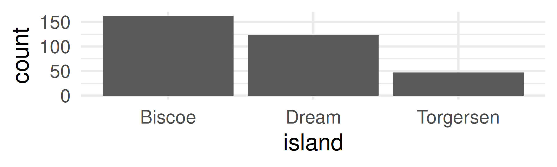
Technically island is cannot be interpreted as a random variable because its values are not numbers, but we also speak about the distribution of the variables.
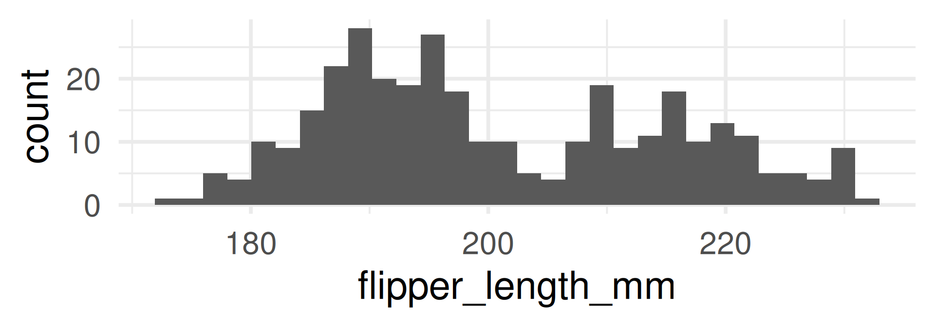
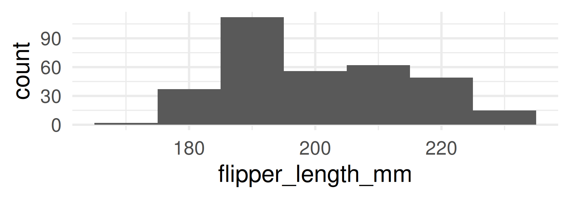
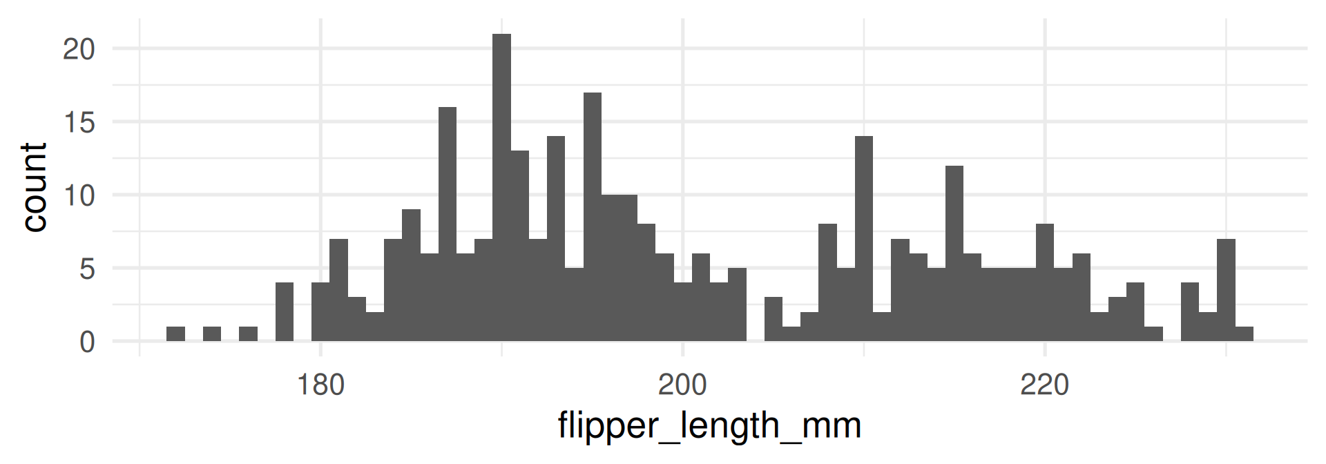
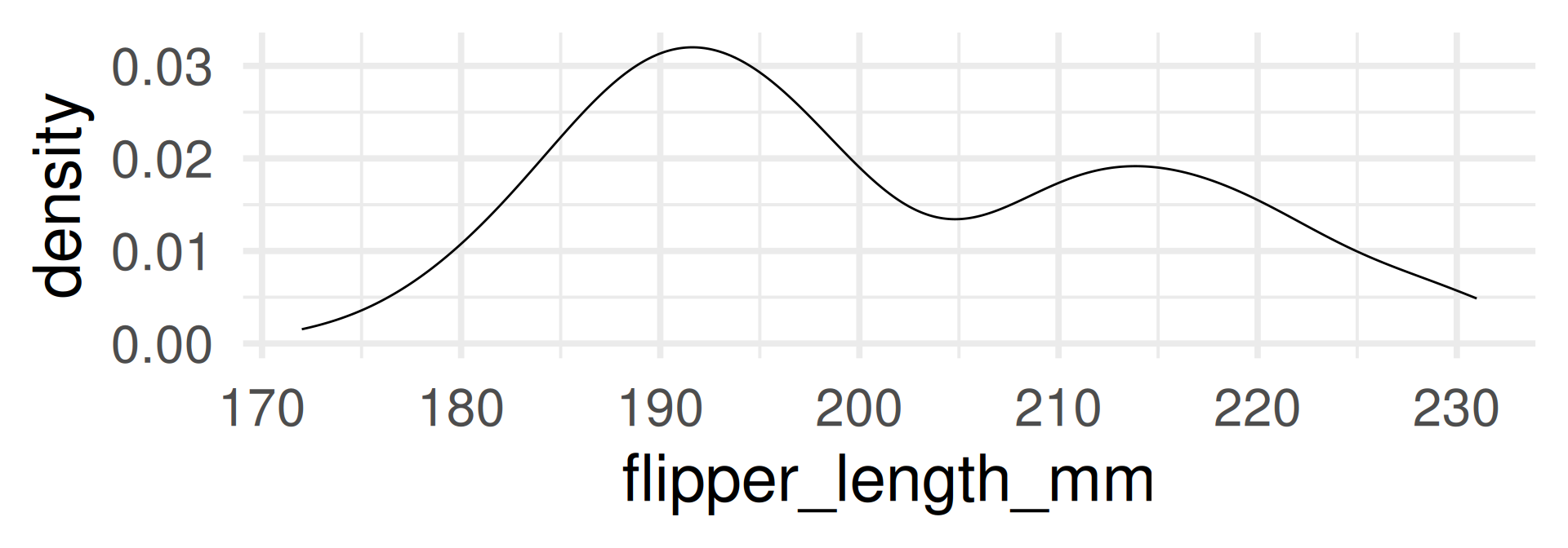
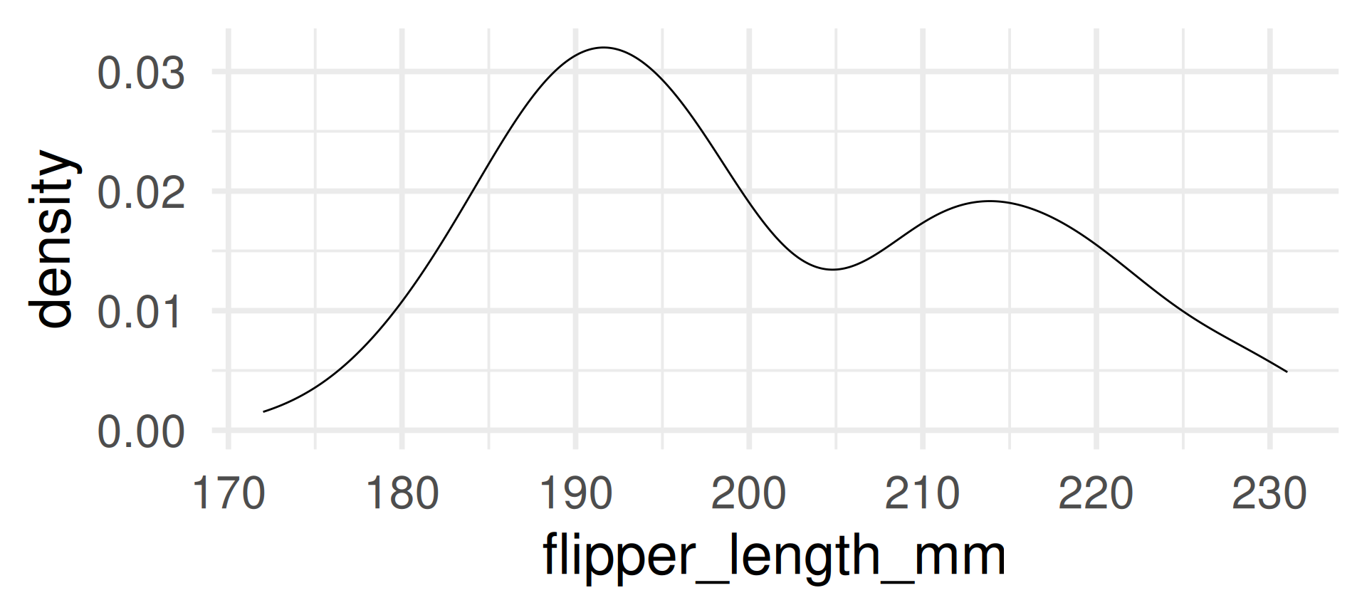
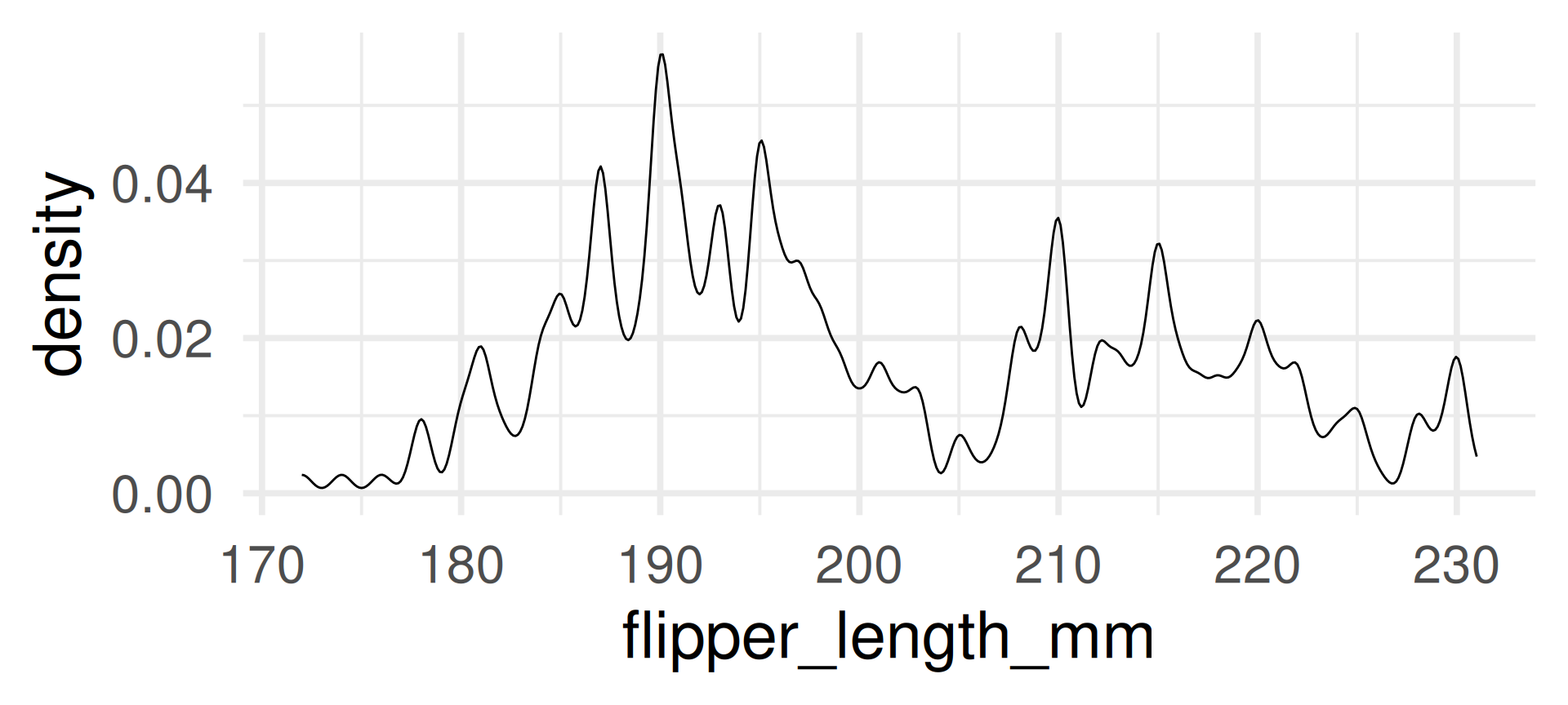
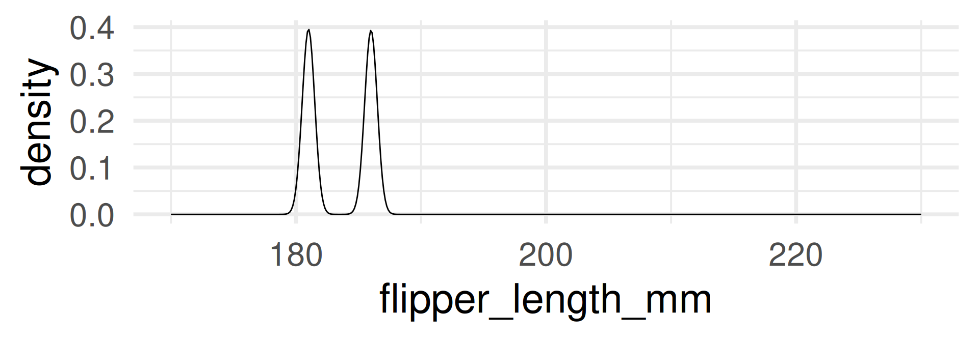
With automatic bandwidth (bw)
A first example for a theoretical random variable.
The number of HEADS in several coin tosses and the number of complications in randomly selected organ donations are examples of random variable which have a binomial distribution.
Definition:
The binomial distribution with parameters \(n\) and \(p\) is
the number of successes in a sequence of \(n\) independent Bernoulli trials
which each delivers a success with probability \(p\) and a failure with probability \((1-p)\).
\[f(k,n,p) = \Pr(k;n,p) = \Pr(X = k) = \binom{n}{k}p^k(1-p)^{n-k}\]
where \(k\) is the number of successes, \(n\) is the number of Bernoulli trials, and \(p\) the success probability.
Probability to have exactly 3 complications in 62 randomly selected organ donations with complication probability \(p=0.1\) is
The probability to have 3 complications or less can be computed as
This was the p-value we computed with simulation for the hypothesis testing example.
For \(X \sim \text{Binom}(n,p)\) (read “\(X\) has a binomial distribution with samplesize \(n\) and success probability \(p\)”)
The expected value of \(X\) is by definition
\[E(X) = \underbrace{\sum_{k = 0}^n k}_{\text{sum over successes}} \cdot \underbrace{\binom{n}{k}p^k(1-p)^{n-k}}_{\text{probability of successes}}\]
Computation shows that \(E(X) = p\cdot n\).
Example: For \(n = 62\) organ donations with complication probability \(p=0.1\), the expected number of complications is \(E(X) = 6.2\).
Compute the p-value:
[1] 0.001455578 0.010027317 0.033981465 0.075514366
[1] 0.1209787
Plotting the probability mass function

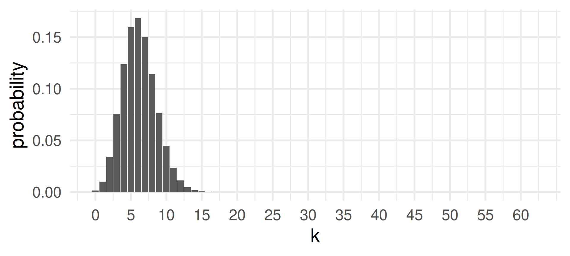
See that the highest probability is achieved for \(k=6\) which is close to the expected value of successes \(E(X) = 6.2\) for \(X \sim \text{Binom}(62,0.1)\).
Changing the sample size \(n\) when the success probability \(p = 0.1\) and the number of successes \(k=3\) is fixed:

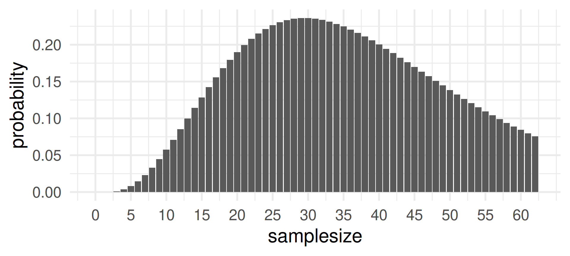
The probability of 3 successes is most likely for sample sizes around 30. Does is make sense?
Yes, because for \(n=30\) the expected value for probability \(p=0.1\) is \(3 = pn = 0.1\cdot 30\).
Changing the sample size \(p\) when the sample size \(n = 62\) and the number of successes \(k=3\) is fixed:

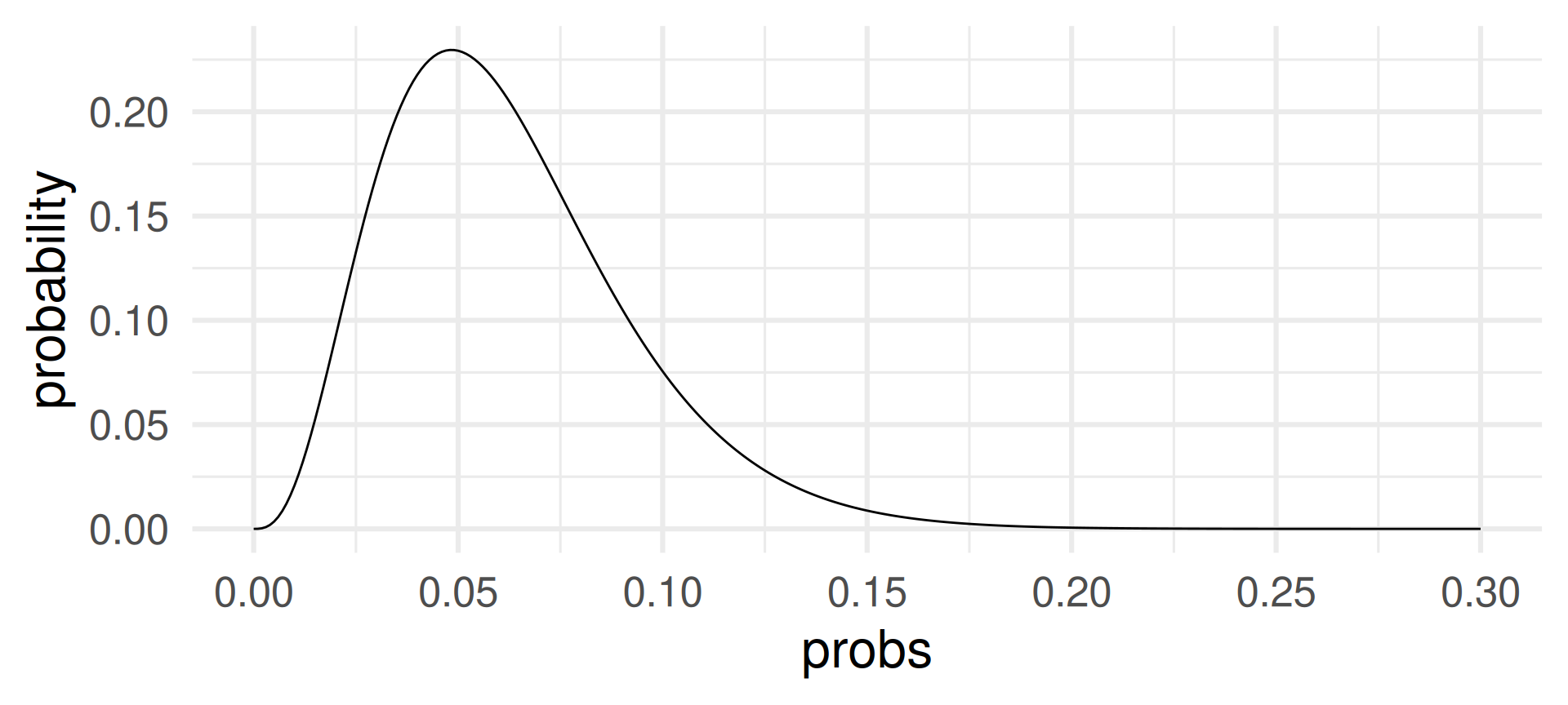
The probability of 3 successes in 62 draws is most likely for success probabilities around 0.05.
For \(p=0.05\) the expected value for \(n=62\) is \(pn = 0.05\cdot 62 = 3.1\).

MDSSB-DSCO-02: Data Science Concepts